Applied Statistics
1MS926, Spring 2019, Uppsala University
©2019 Raazesh Sainudiin. Attribution 4.0 International (CC BY 4.0)
04. Conditional Probability, Random Variables, Loops and Conditionals
Topics:
- Probability
- Independence
- Conditional Probability
- Bayes Theorem
- Random Variables
- For loops
- Conditional Statements
- List Comprehensions
- Anonymous Functions
Probability
Recap on probability
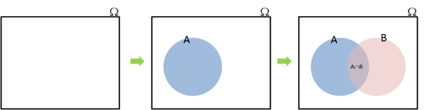
An experiment is an activity or procedure that produces distinct or well-defined outcomes. The set of such outcomes is called the sample space of the experiment. The sample space is usually denoted with the symbol $\Omega$.
An event is a subset of the sample space.
Probability is a function that associates each event in a set of events (denoted by $\{ \text{ events }\}$) with a real number in the range 0 to 1 (denoted by $[0,1]$):
$$P : \{ \text{ events } \} \rightarrow [0,1]$$
while satisfying the following axioms:
- For any event $A$, $ 0 \le P(A) \le 1$.
- If $\Omega$ is the sample space, $P(\Omega) = 1$.
- If $A$ and $B$ are disjoint (i.e., $A \cap B = \emptyset$), then $P(A \cup B) = P(A) + P(B)$.
- If $A_1, A_2, \ldots$ is an infinite sequence of pair-wise disjoint events (i.e., $A_i \cap A_j = \emptyset$ when $i \ne j$), then $$ \begin{array}{lcl} \underbrace{P\left(\bigcup_{i=1}^{\infty}A_i\right)} &=& \underbrace{\sum_{i=1}^{\infty}P\left(A_i\right)} \\ A_1 \cup A_2 \cup A_3 \dots &=& P(A_1) + P(A_2) + P(A_3) + \ldots \end{array} $$
Property 1
$P(A) = 1 - P(A^c)$, where $A^c = \Omega \setminus A$
Property 2
For any two events $A$, $B$,
$P(A \cup B) = P(A) + P(B) - P(A \cap B)$
The idea in Property 2 generalises to the inclusion-exclusion formula as follows:
Let $A_1, A_2, \ldots, A_n$ be any $n$ events. Then,
$$ \begin{array}{lcl} P\left(\bigcup_{i=1}^n A_i \right) &=& \sum_{i=1}^nP(A_i) \, - \, \sum_{i<j}P(A_i \cap A_j) \\ &\,& \quad + \, \sum_{i<j<k}P(A_i \cap A_j \cap A_k) + \ldots + (-1)^{n+1}P(A_1 \cap A_2 \cap \ldots \cap A_n) \end{array} $$
In words, we take all the possible intersections of one, two, three, $\ldots$, $n$ events and let the signs alternate to more carefully account for multiple countings.
Question
Does the inclusion-exclusion formula agree with the extended Axiom 3: If $A_1, A_2, \ldots, A_n$ are pair-wise disjoint events then $P\left( \bigcup_{i=1}^n A_i \right) = \sum_{i=1}^nP(A_i)$?
The domain of the probability function
What exactly is stipulated by the axioms about the domain of the probability function?
The domain should be a sigma-field ($\sigma$-field) or sigma-algebra ($\sigma$-algebra), denoted $\sigma(\Omega)$ or $\mathcal{F}$ such that:
- $\Omega \in \, \mathcal{F}$
- $ A \in \mathcal{F} \Rightarrow A^c \in \, \mathcal{F}$
- $A_1, A_2, \ldots \in \mathcal{F} \Rightarrow \cup A_i \in \, \mathcal{F}$
We will not use the full machinery of sigma-algebras in this course as it requires more formal training in mathemtics but it is important to know what's under the hood of the domain of our probability function; in case we need to dive deeper into sigma-algebras for more compicated probabilistic models of our data.
def showURL(url, ht=500):
    """Return an IFrame of the url to show in notebook with height ht"""
    from IPython.display import IFrame
    return IFrame(url, width='95%', height=ht)
showURL('https://en.wikipedia.org/wiki/Sigma-algebra',600)
Probability Space
Thus the domain of the probability is not just any old set of events (recall events are subsets of $\Omega$), but rather a set of events that form a $\sigma$-field that contains the sample space $\Omega$, is closed under complementation and countable union.
$\left(\Omega, \mathcal{F}(\Omega), P\right)$ is called a probability space or probability triple.
Example
Let $\Omega = \{H, T\}$. What $\sigma$-fields could we have?
$\mathcal{F}\left({\Omega}\right) = \{\{H, T\}, \emptyset, \{H\}, \{T\}\}$ is the finest $\sigma$-field.
$\mathcal{F}'\left({\Omega}\right) = \{ \{H, T\}, \emptyset \}$ is a trivial $\sigma$-field.
Example
Let $\Omega = \{\omega_1, \ldots, \omega_n\}$.
$\mathcal{F}\left({\Omega}\right) = 2^\Omega$, the set of all subsets of $\Omega$, also known as the power set of $\Omega$.
$\vert 2^\Omega \vert = 2^n$.
We have finally defined probability space as quickly as possible from first principles. As your mathematical background matures you can dive deeper into more subtle aspects of probability space, in its generality, as needed.
These examples are great for becoming more familiar with probability spaces.
showURL("https://en.wikipedia.org/wiki/Probability_space",400)
Independence
Two events $A$ and $B$ are independent if $P(A \cap B) = P(A)P(B)$.
Intuitively, $A$ and $B$ are independent if the occurrence of $A$ has no influence on the probability of the occurrence of $B$ (and vice versa).
Example
Flip a fair coin twice. Event $A$ is the event "The first flip is 'H'"; event $B$ is the event "The second flip is 'H'".
$P(A) = \frac{1}{2}$, $P(B) = \frac{1}{2}$
Because the flips are independent (what happens on the first flip does not influence the second flip),
$P(A \cap B) = \frac{1}{2} \times \frac{1}{2} = \frac{1}{4}$.
Example
We can generalise this by saying that we will flip a coin with an unknown probability parameter $\theta \in [0,1]$. We flip this coin twice and the coin is made so that for any flip, $P(\mbox{'H'}) = \theta$, $P(\mbox{'T'}) = 1-\theta$.
Take the same events as before: event $A$ is the event "The first flip is 'H'"; event $B$ is the event "The second flip is 'H'".
Because the flips are independent,
$P(A \cap B) = \theta \times \theta = \theta^2$.
If we take event $C$ as the event "The second flip is 'T'", then
$P(A \cap C) = \theta \times (1-\theta)$.
Example
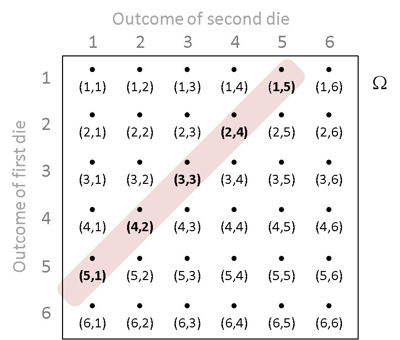
Roll a fair die twice. The face of the die is enumerated 1, 2, 3, 4, 5, 6.
Event $A$ is the event "The first roll is 5"; event $B$ is the event "The second roll is 1".
$P(A) = \frac{1}{6}$, $P(B) = \frac{1}{6}$
If the two rolls are independent,
$P(A \cap B) = \frac{1}{6} \times \frac{1}{6} = \frac{1}{36}$
You try at home
For those who are rusty on probability models.
Suppose you roll two fair dice independently. What is the probability of getting the sum of the outcomes to be seven?
Solution: Watch the Khan Academy movie about probability and two dice.
Conditional probability
Suppose that we are told that the event $A$ with $P(A) > 0$ occurs and we are interested in whether another event $B$ will now occur. The sample space has shrunk from $\Omega$ to $A$. The probability that event $B$ will occur given that $A$ has already occurred is defined by
$$P(B|A) = \frac{P(B \cap A)}{P(A)}$$
We can understand this by noting that
Only the outcomes in $B$ that also belong to $A$ can possibly now occur, and Since the new sample space is $A$, we have to divide by $P(A)$ to make $$P(A|A) = \frac{P(A \cap A)}{P(A)} = \frac{P(A)}{P(A)} = 1$$ If the two events $A$ and $B$ are independent then
$$P(B|A) = \frac{P(B \cap A)}{P(A)} = \frac{P(B)P(A)}{P(A)} = P(B)$$
which makes sense - we said that if two events are independent, then the occurrence of $A$ has no influence on the probability of the occurrence of $B$.
Example
Roll two fair dice.
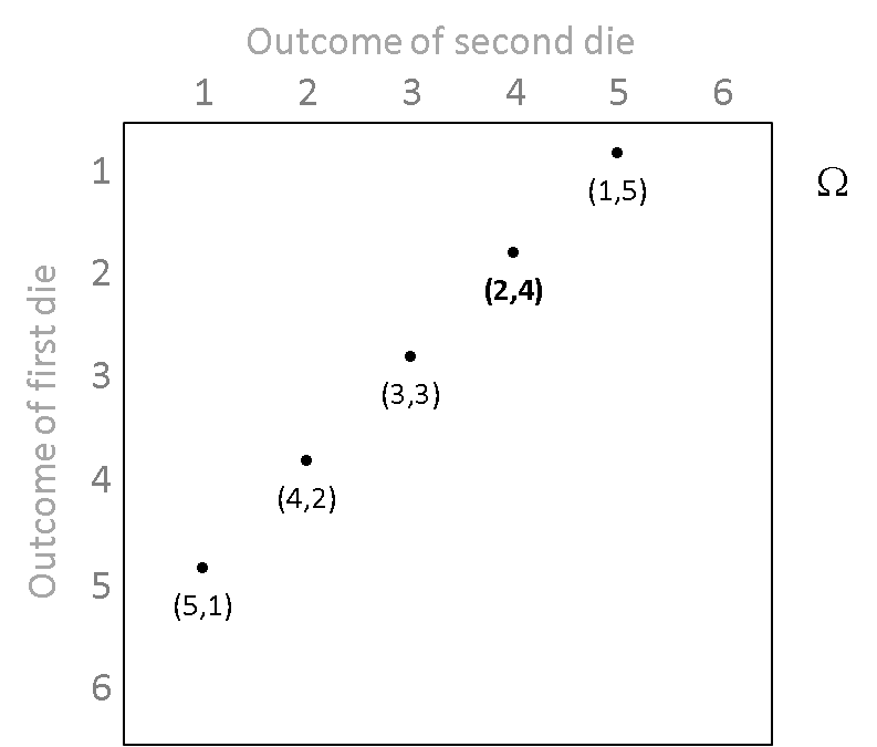
Event $A$ is the event "The sum of the dice is 6"; event $B$ is the event "The first die is 2".
How many ways can we get a 6 out of two dice?
$A = \{(1,5), (2,4), (3,3), (4,2), (5,1)\}$
$P(A) = \frac{1}{36} + \frac{1}{36} + \frac{1}{36} + \frac{1}{36} + \frac{1}{36} = \frac{5}{36}$
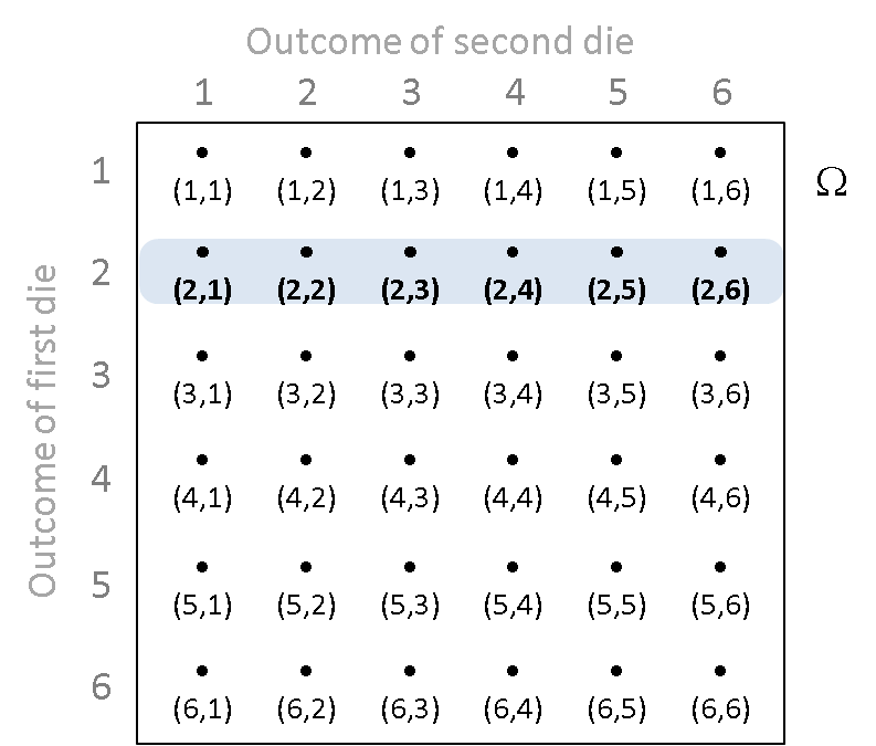
$B = \{(2,1), (2,2), (2,3), (2,4), (2,5), (2,6)\}$
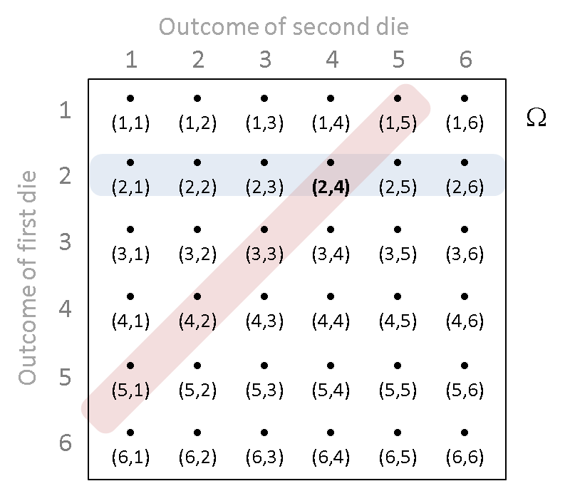
$B \cap A = \{ (2,4)\}$
$P(B \cap A) = \frac{1}{36}$
$P(B|A) = \frac{P(B \cap A)}{P(A)} = \frac{\frac{1}{36}}{\frac{5}{36}} = \frac{1}{5}$
Look at this result in terms of what we said about the sample space shrinking to $A$.
Bayes Theorem
We just saw that $P(B|A)$, the conditional probability that event $B$ will occur given that $A$ has already occurred is defined by $P(B \cap A)/P(A)$. By using the fact that $B \cap A = A \cap B$ and reapplying the definition of conditional probability to $P(A|B)=P(A \cap B)/P(B)$, we get the so-called Bayes theorem.
$$\boxed{P(B|A) = \frac{P(B \cap A)}{P(A)} = \frac{P(A \cap B)}{P(A)} = \frac{P(A|B) P(B)}{P(A)}}$$
You try at home
Suppose we have a bag of ten coins. Nine of the ten coins are fair but one of the coins has heads on both sides. What is the probability of getting five heads in a row if I picked a coin at random from the bag and flipped it five times? If I obtained five heads in a row by choosing a coin out of the bag at random and flipping it five times, then what is the probability that I have picked the two-headed coin?
Solution: Watch the Khan Academy movies about applications of conditional probability and Bayes theorem to this bag of 10 coins.
Consider the experiment where we roll two fair dice independently.
Let $D$ be the event that "the sum of the two dice is 8" and let $C$ be the event that "the first die is 2".
What is the probability of D given C, i.e. what is $P(D|C)$?
Do the calculation by hand and write the answer in the next cell by assigning the variable ProbOfDGivenC.
# Replace XXX below with the correct answer to Assignment 1 Problem 3
# Do NOT change the name of the variable ProbOfDGivenC
ProbOfDGivenC = XXX
Local Test for Assignment 1, PROBLEM 3
Evaluate cell below to make sure your answer is valid. You should not modify anything in the cell below when evaluating it to do a local test of your solution.
# test that your answer is indeed a probability by evaluating this cell after you replaced XXX above and evaluated it.
try:
    assert(ProbOfDGivenC >= 0 and ProbOfDGivenC <= 1)
    print("Your answer is a probability, hopefully it is correct.")
except AssertionError:
    print("Try again! and make sure you are actually producing a valid probability, i.e., a real number in [0,1]")
A foretaste of simulation
The next cell uses a function called randint which we will talk about more later in the course. For this week we'll just use randint as a computerised way of rolling a die: every time we call randint(1,6) we will get some integer number from 1 to 6, we won't be able to predict in advance what we will get, and the probability of each of the numbers 1, 2, 3, 4, 5, 6 is equal. Here we use randint to simulate the experiment of tossing two dice. The sample space $\Omega$ is all 36 possible ordered pairs $(1,1), \ldots (6,6)$. We print out the results for each die. Try evaluating the cell several times and notice how the numbers you get differ each time.
randint?
# evaluate this cell again to see the random outcomes change
die1 = randint(1,6)
die2 = randint(1,6)
print "(die 1, die2) is (", die1, ", ", die2, ")"
Random Variables
A random variable is a mapping from the sample space $\Omega$ to the set of real numbers $\mathbb{R}$. In other words, it is a numerical value determined by the outcome of the experiment. (Actually, this is a real-valued random variable and one can have random variables taking values in other sets).
This is not as complicated as it sounds: let's look at a simple example:
Example
Roll two fair dice.
The sample space is the set of 36 ordered pairs $\Omega = \{(1,1), (1,2), \dots, (2,1), (2,2), \ldots, (1,6), \ldots, (6,6)\}$
Let random variable $X$ be the sum of the two numbers that appear, $X : \Omega \rightarrow \mathbb{R}$.
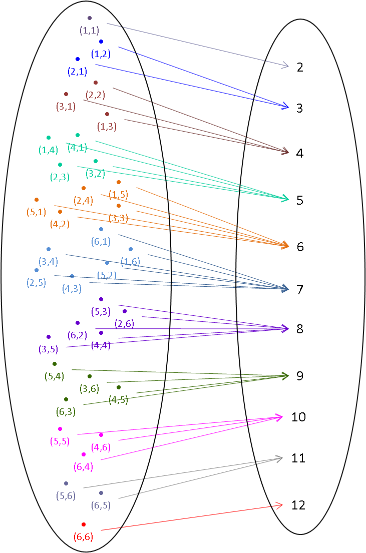
For example, $X\left(\{(6,6)\}\right) = 12$
$P(X=12) = P\left(\{(6,6)\}\right)$
And, $X\left( \{ (3,2) \}\right) = 5$
Formal definition of a random variable
Let $\left(\Omega, \mathcal{F}, P \right)$ be some probability triple. Then a random variable, say $X$, is a function from the sample space $\Omega$ to the set of real numbers $\mathbb{R}$
$$X: \Omega \rightarrow \mathbb{R}$$
such that for every number $x$ in $\mathbb{R}$, the inverse image of the half-open interval $(-\infty, x]$ is an element of the collection of events $\mathcal{F}$, i.e.,
for every number $x$ in $\mathbb{R}$, $$X^{[-1]}\left( (-\infty, x] \right) := \{\omega: X(\omega) \le x\} \in \mathcal{F}$$
Discrete random variable
A random variable is said to be discrete when it can take a countable sequence of values (a finite set is countable). The three examples below are discrete random variables.
Probability of a random variable
Finally, we assign probability to a random variable $X$ as follows:
$$P(X \le x) = P \left( X^{[-1]}\left( (-\infty, x] \right) \right) := P\left( \{ \omega: X(\omega) \le x \} \right)$$
Distribution Function
The distribution function (DF) or cumulative distribution function (CDF) of any RV $X$, denoted by $F$ is:
$$F(x) := P(X \leq x) = P\left( \{ \omega: X(\omega) \leq x \} \right) \mbox{, for any } x \in \mathbb{R}$$
Example - Sum of Two Dice
In our example above (tossing two die and taking $X$ as the sum of the numbers shown) we said that $X\left((3,2)\right) = 5$, but (3,2) is not the only outcome that $X$ maps to 5: $X^{[-1]}\left(5\right) = \{(1,4), (2,3), (3,2), (4,1)\}$
$$ \begin{array}{lcl} P(X=5) & = & P\left(\{\omega: X(\omega) = 5\}\right)\\ & = & P\left(X^{[-1]}\left(5\right)\right)\\ & = & P(\{(1,4), (2,3), (3,2), (4,1)\}) \end{array} $$
Example - Pick a Fruit at Random
Remember our "well-mixed" fruit bowl containing 3 apples, 2 oranges, 1 lemon? If our experiment is to take a piece of fruit from the bowl and the outcome is the kind of fruit we take, then we saw that $\Omega = \{\mbox{apple}, \mbox{orange}, \mbox{lemon}\}$.
Define a random variable $Y$ to give each kind of fruit a numerical value: $Y(\mbox{apple}) = 1$, $Y(\mbox{orange}) = 0$, $Y(\mbox{lemon}) = 0$.
Example - Flip Until Heads
Flip a fair coin until a 'H' appears. Let $X$ be the number of times we have to flip the coin until the first 'H'.
$\Omega = \{\mbox{H}, \mbox{TH}, \mbox{TTH}, \ldots, \mbox{TTTTTTTTTH}, \ldots \}$
$X(\mbox{H}) = 0$, $X(\mbox{TH}) = 1$, $X(\mbox{TTH}) = 2$, $\ldots$
You try at home
Consider the example above of 'Pick a Fruit at Random'. We defined a random variable $Y$ there as $Y(\mbox{apple}) = 1$, $Y(\mbox{orange}) = 0$, $Y(\mbox{lemon}) = 0$. Using step by step arguments as done in the example of 'Sum of Two Dice' above, find the following probabilities for our random variable $Y$: $$ \begin{array}{lcl} P(Y=0) & = & P\left(\{\omega: Y(\omega) = \quad \}\right)\\ & = & P\left(Y^{[-1]} \left( \quad \right)\right)\\ &= & P(\{\quad , \quad \}) \end{array} $$
Watch the Khan Academy movie about random variables
When we introduced the subject of probability, we said that many famous people had become interested in it from the point of view of gambling. Games of dice are one of the earliest forms of gambling (probably deriving from an even earlier game which involved throwing animal 'ankle' bones or astragali). Galileo was one of those who wrote about dice, including an important piece which explained what many experienced gamblers had sensed but had not been able to formalise - the difference between the probability of throwing a 9 and the probability of throwing a 10 with two dice. You should be able to see why this is from our map above. If you are interested you can read a translation (Galileo wrote in Latin) of Galileo's Sorpa le Scoperte Dei Dadi. This is also printed in a nice book, Games, Gods and Gambling by F.N. David (originally published 1962, newer editions now available).
Implementing a Random Variable
We have made our own random variable map object in Sage called RV. As with the Sage probability maps we looked at last week, it is based on a map or dictionary. We specify the sample the samplespace and probabilities and the random variable map, MapX, from the samplespace to the values taken by the random variable $X$).
# create a class for a random variable map - just evaluate this cell and don't worry about understanding this now
# This was coded by Jenny Harlow

class RV(object):                # class definition
    'Random variable class'
    def __init__(self, sspace=[], probs=[], probmap=None, values=[]): # constructor with default args

        # provide default empty values which will be used if initialisation fails in try clause
        self.__rvmap = {}  # if error, rvmap is empty
        self.__rvinvmap = {}  # if error, rvinvmap is empty
        self.__rvprobmap = {}  # if error, rvprobmap is empty
        self.__lastvalue = None     # for the last value for which a probability was calculated

        try: # make checks on the objects given as sspace and probs
            if probmap == None: # no probability map provided
               self.__probmap = ProbyMap(sspace=sspace, probs=probs) # make the probability map

            else:
                assert isinstance(probmap, ProbyMap) # make sure probmap is a ProbyMap
                self.__probmap = probmap # use the provided probability map
                sspace=[]
                for ev in self.__probmap.ref_probmap.keys():
                    sspace.append(ev)
            values_list = list(values) # make values into a list
            assert len(self.__probmap.ref_probmap.keys()) == len(values_list) # 1 value for each event

            # if there has been no error make the rv map as private
            self.__rvmap = dict(zip(list(sspace),values_list))
                                        # map from sspace to random variable values

            self.__rvinvmap = {} # make an empty map for inverse map from rvs to lists of events
            self.__rvprobmap = {} # and an empty map for the map from rvs to probabilities
            for ev in self.__rvmap: # fill in the inverse map and rvmap
                if self.__rvmap[ev] in self.__rvinvmap.keys(): # if the rv already there
                    self.__rvinvmap[self.__rvmap[ev]].append(ev) # add the event to list
                    self.__rvprobmap[self.__rvmap[ev]].append(self.__probmap.ref_probmap[ev]) # add proby
                else:
                    self.__rvinvmap[self.__rvmap[ev]] = [ev, ] # add entry
                    self.__rvprobmap[self.__rvmap[ev]] = [self.__probmap.ref_probmap[ev], ] # add entry

        except AssertionError:
            print "Check your sample space, probabilities and random variable values"
        except TypeError, diag:
            print str(diag)


    def __str__(self):                            # redefine printable string rep
        'Printable representation of the object.'
        return "Inverse map from RV to events is " + str(self.__rvinvmap)


    __repr__ = __str__

    def __printprobs(self): # method to create a printable representation of the rv probababilities
        'Printable representation of the probabilities.'
        num_keys = len(self.__rvprobmap.keys())
        counter1 = 0
        retval = 'RV probabilites map is {'
        for each_key in self.__rvprobmap:
            counter1 += 1
            retval += str(each_key)
            retval += ': ['
            num_vals = len(self.__rvprobmap[each_key])
            counter2 = 0
            for val in self.__rvprobmap[each_key]:
                counter2 += 1
                retval += "%.3f" % val
                if counter2 < num_vals:
                    retval += ', '
            retval += ']'
            if counter1 < num_keys:
                retval += ', '
        retval += '}'
        return retval

    def get_probmap(self):                        # get a deep copy of the probmap
        return copy.deepcopy(self.__probmap)      # getter cannot alter object's map

    def get_rvmap(self):                          # get a deep copy of the rv map
        return copy.deepcopy(self.__rvmap)        # getter cannot alter object's map

    def get_rvinvmap(self):                          # get a deep copy of the rvinv map
        return copy.deepcopy(self.__rvinvmap)        # getter cannot alter object's map

    def get_rvprobmap(self):                          # get a deep copy of the rv prob map
        return copy.deepcopy(self.__rvprobmap)        # getter cannot alter object's map

    probmap = property(get_probmap)
    rvmap = property(get_rvmap)
    rvinvmap = property(get_rvinvmap)
    rvprobmap = property(get_rvprobmap)


    def __pow__(self, x):
        '''random variable exponentiated.'''
        try:
            # proby map is going to be this object's proby map
            newvalues = [] # empty list for new values
            for ev in self.__probmap.ref_probmap: # for each event
                oldval = self.__rvmap[ev]         # find the value the event maps to
                newval = oldval^x                 # take the function of the value
                newvalues.append(newval)          # add the function of the value to the list of values

            self.__lastvalue = 'X'                # set the last calculation attribute on this RV to 'X'
            return RV(probmap=self.__probmap, values=newvalues)

        except TypeError:
            print "Cannot raise to power " + str(x)
            return None

    def __add__(self, x):
        '''random variable with number added.'''
        try:
            # proby map is going to be this object's proby map
            newvalues = [] # empty list for new values
            for ev in self.__probmap.ref_probmap: # for each event
                oldval = self.__rvmap[ev]         # find the value the event maps to
                newval = oldval+x                 # take the function of the value
                newvalues.append(newval)          # add the function of the value to the list of values

            self.__lastvalue = 'X'                # set the last calculation attribute on this RV to 'X'
            return RV(probmap=self.__probmap, values=newvalues)

        except TypeError:
            print "Cannot add" + str(x)
            return None

    __radd__ = __add__         # adding object to number is same as adding number to object

    def __sub__(self, x):
        '''random variable with number substracted.'''
        try:
            # proby map is going to be this object's proby map
            newvalues = [] # empty list for new values
            for ev in self.__probmap.ref_probmap: # for each event
                oldval = self.__rvmap[ev]         # find the value the event maps to
                newval = oldval-x                 # take the function of the value
                newvalues.append(newval)          # add the function of the value to the list of values

            self.__lastvalue = 'X'                # set the last calculation attribute on this RV to 'X'
            return RV(probmap=self.__probmap, values=newvalues)

        except TypeError:
            print "Cannot substract" + str(x)
            return None

    def __rsub__(self, x):
        '''number with random variable number substracted.'''
        try:
            # proby map is going to be this object's proby map
            newvalues = [] # empty list for new values
            for ev in self.__probmap.ref_probmap: # for each event
                oldval = self.__rvmap[ev]         # find the value the event maps to
                newval = x-oldval                 # take the function of the value
                newvalues.append(newval)          # add the function of the value to the list of values

            self.__lastvalue = 'X'                # set the last calculation attribute on this RV to 'X'
            return RV(probmap=self.__probmap, values=newvalues)

        except TypeError:
            print "Cannot substract rv from " + str(x)
            return None

    def __mul__(self, x):
        '''random variable multiplied by number.'''
        try:
            # proby map is going to be this object's proby map
            newvalues = [] # empty list for new values
            for ev in self.__probmap.ref_probmap: # for each event
                oldval = self.__rvmap[ev]         # find the value the event maps to
                newval = oldval*x                 # take the function of the value
                newvalues.append(newval)          # add the function of the value to the list of values

            self.__lastvalue = 'X'                # set the last calculation attribute on this RV to 'X'
            return RV(probmap=self.__probmap, values=newvalues)

        except TypeError:
            print "Cannot multiply by " + str(x)
            return None

    __rmul__ = __mul__      # object multiplied by number is same as number multiplied by object

    def __div__(self, x):
        '''random variable divided  by number.

        This performs true division.'''
        try:
            # proby map is going to be this object's proby map
            newvalues = [] # empty list for new values
            for ev in self.__probmap.ref_probmap: # for each event
                oldval = self.__rvmap[ev]         # find the value the event maps to
                newval = oldval/float(x)          # take the function of the value
                newvalues.append(newval)          # add the function of the value to the list of values

            self.__lastvalue = 'X'                # set the last calculation attribute on this RV to 'X'
            return RV(probmap=self.__probmap, values=newvalues)

        except TypeError:
            print "Cannot divide by " + str(x)
            return None

    def P(self, myval):
        '''Return the probability of a value.'''
        self.__lastvalue = None     # reset attribute lastvalue
        retval = 0     # default return value
        try:
            assert myval in self.__rvprobmap.keys()
            retval = sum(self.__rvprobmap[myval])
            self.__lastvalue = myval     # set lastvalue to the value we just calculated proby for
                                         # last value is used by explainLastCalc method

        except TypeError, diag:
            print str(diag)

        except AssertionError:
            retval = 0
        return retval

    def explainLastCalc(self):  # return details of the calculation for the last probability calculated
        if self.__lastvalue == 'X':
            retvalue = "Sorry, that calculation was on function of this RV, not the RV itself"
        elif self.__lastvalue == None:
            retvalue = "Sorry, no valid last calculation to explain"
        elif self.__lastvalue == 'E':
            try:
                num_keys = len(self.__rvprobmap.keys())
                counter = 0
                retvalue = str(self)
                retvalue += ' and \n'
                retvalue += self.__printprobs()
                retvalue += '\nso E()'
                retvalue += ' = '
                for val in self.__rvprobmap:
                    retvalue += "(%.1f" % val
                    retvalue += ' multiplied by '
                    retvalue += "%.3f" % sum(self.__rvprobmap[val])
                    retvalue += ')'
                    counter+=1
                    if counter < num_keys:
                        retvalue += '\n+ '
                retvalue += '\nwhich is '
                retvalue += "%.2f" % self.Exp()
            except TypeError, diag:
                retvalue = "Error, " + str(diag)
        elif self.__lastvalue == 'V':
            try:
                num_keys = len(self.__rvprobmap.keys())
                counter = 0
                mean = self.Exp()
                retvalue = str(self)
                retvalue += ' and \n'
                retvalue += self.__printprobs()
                retvalue += '\nso Var()'
                retvalue += ' = '
                for val in self.__rvprobmap:
                    retvalue += "((%.1f - %.2f)^2" % (val, mean)
                    retvalue += ' multiplied by '
                    retvalue += "%.3f" % sum(self.__rvprobmap[val])
                    retvalue += ')'
                    counter+=1
                    if counter < num_keys:
                        retvalue += '\n+ '
                retvalue += '\n'
                retvalue += "where %.2f is the mean," % mean
                retvalue += '\nso the variance is '
                retvalue += "%.2f" % self.Variance()
            except TypeError, diag:
                retvalue = "Error, " + str(diag)
        else:
            try:
                retvalue = str(self)
                retvalue += ' and \n'
                retvalue += self.__printprobs()
                retvalue += '\nso P('
                retvalue += str(self.__lastvalue)
                retvalue += ') = '
                retvalue += ' the sum of the probabilities '
                retvalue += str(self.__lastvalue)
                retvalue += ' maps to, which is '
                retvalue += "%.2f" % self.P(self.__lastvalue)
            except TypeError, diag:
                retvalue = "Error: Probably invalid value"

        print retvalue


    def Exp(self):
        '''Return the expectation of this RV.'''
        self.__lastvalue = None     # reset attribute lastvalue
        retval = 0     # default return value
        try:
            for val in self.__rvprobmap:
                retval += val * sum(self.__rvprobmap[val])
            self.__lastvalue = 'E'     # set attribute lastvalue
        except TypeError, diag:
            print str(diag)
            retval = None

        return float(retval)

    def Variance(self):
        '''Return the variance of this RV.'''
        self.__lastvalue = None     # reset attribute lastvalue
        retval = 0     # default return value
        try:
            for val in self.__rvprobmap:
                retval += val^2 * sum(self.__rvprobmap[val])
            retval = retval - (self.Exp())^2
            self.__lastvalue = 'V'     # set attribute lastvalue
        except TypeError, diag:
            print str(diag)
            retval = None

        return float(retval)

# the class has ended here, now we have definitions outside the class

def E(obj):
    try:
        assert isinstance(obj, RV)
        retvalue = obj.Exp()
    except AssertionError:
        print "Sorry: can only do expectations on RVs"
        retvalue = None
    return retvalue

def Var(obj):
    try:
        assert isinstance(obj, RV)
        retvalue = obj.Variance()
    except AssertionError:
        print "Sorry: can only do variances on RVs"
        retvalue = None
    return retvalue

# create a class for a probability map - if you are new to SageMath/Python just evaluate and skip this cell
# This was coded by Jenny Harlow

import copy
class ProbyMap(object):                # class definition
    'Probability map class'
    def __init__(self, sspace, probs): # constructor
        self.__probmap = {}  # default probmap is empty
        # make checks on the objects given as sspace and probs
        try:
            sspace_set = set(sspace) # check that we can make the sample space into a set
            assert len(sspace_set) == len(sspace) # and not lose any elements
            prob_list = list(probs) # and we can make the probs into a list
            probsum = sum(prob_list) # and we can sum the probs
            assert probsum == 1 # and the probs sum to 1
            assert len(prob_list) == len(sspace_set) # and there is proby for each event

            self.__probmap = dict(zip(list(sspace),prob_list))    # map from sspace to probs

        except TypeError, diag: # if there any problems with types
            init_error = 1
            print str(diag)

        except AssertionError:
            init_error = 1
            print "Check sample space and probabilities"


    def P(self, events):
        '''Return the probability of an event or set of events.

        events is set of events in the sample space to calculate the probability for.'''

        retvalue = 0
        try:
            events_set = set(events) # check we can make a set out of the events
            assert len(events_set) == len(events) # and not lose any events
            assert events_set <= set(self.__probmap.keys()) # events subset of sample space

            for ev in events:     # add each mapped probability to the return value
                retvalue += self.__probmap[ev]

        except TypeError, diag:
            print str(diag)

        except AssertionError:
            print "Check your events"

        return retvalue

    def __str__(self):                            # redefine printable string rep
        'Printable representation of the object.'
        num_keys = len(self.__probmap.keys())
        counter = 0
        retval = '{'
        for each_key in self.__probmap:
            counter += 1
            retval += str(each_key)
            retval += ': '
            retval += "%.3f" % self.__probmap[each_key]
            if counter < num_keys:
                retval += ', '
        retval += '}'

        return retval

    __repr__ = __str__

    def get_probmap(self):                        # get a deep copy of the proby map
        return copy.deepcopy(self.__probmap)      # getter cannot alter object's map

    probmap = property(get_probmap)               # allow read access via .probmap

    def get_ref_probmap(self):                    # get a reference to the real probmap
        return self.__probmap                     # getter can alter the object's map


    ref_probmap = property(get_ref_probmap)       # allow access via .ref_probmap

    @staticmethod
    def dictExp(big_map, small_map):
        '''Internal helper function for __pow__(...).

        Takes two proby map dictionaries and returns one mult by other.'''
        new_bl = {}
        for sle in small_map:
            for ble in big_map:
                new_key = str(ble) + ' ' + str (sle)
                new_bl[new_key] = big_map[ble]*small_map[sle]
        return new_bl

    def __pow__(self, x):
        '''probability map exponentiated.'''
        try:
            assert isinstance(x, Integer)
            pmap = copy.deepcopy(self.__probmap) # copy the probability map dictionary
            new_pmap = copy.deepcopy(self.__probmap) # and another copy
            for i in range(x-1):
                new_pmap = self.dictExp(new_pmap, pmap)

            return ProbyMap(new_pmap.keys(), new_pmap.values())

        except AssertionError:
            print "cannot raise to non-integer power"
            return None
Example 1: fruit bowl experiments
We are going to use our class 'RV' above and the fruit bowl example, and the random variable $X$ to give each kind of fruit a numerical value: $X(\mbox{apple}) = 1$, $X(\mbox{orange}) = X(\mbox{lemon}) = 0$ This is a discrete random variable because it can only take a finite number of discrete values (in this case, either 1 or 0).
(You don't have to worry about how RV works: it is our 'home-made' class for you to try out.)
# the sample space set as a list of outcomes
samplespace = ['apple', 'orange', 'lemon']
# the corresponding list of outcome probabilities
probabilities = [3/6, 2/6, 1/6]
# list of image values corresponding to the list of outcomes
# taken by the random variable X (1 if we pick an apple and 0 otherwise)
mapX = [1, 0, 0]
print "defined samplespace, probabilities, and mapX"
To make an RV, we can specify the lists for the sample space, the probabilities, and the random variable values associated with each outcome. Since there are three different lists here, we can make things clearer by actually saying what each list is. The RV we create in the cell below is going to be called X.
X = RV(sspace=samplespace, probs=probabilities, values=mapX) # this random variable will be called X
X # disclose the representation of the random variable X
We can get probabilities using the syntax X.P(x) to find $P(X=x)$.
X.P(1) # find the probability that X is 1
X.explainLastCalc() # print out the values used in the calculation of the probability that X = 1
You have seen that different random variables can be defined on the same probability space, i.e., the sample space and the associated probability map, depending on how the outcomes are mapped to real values taken by the random variable. Usually there is some good experimental or mathematical reason for the particular random variable (i.e., event-to-value-mappings) that we use. In the experiment we just did we could have been an experimenter particularly interested in citrus fruit but not concerned with what particular kind of citrus it is.
On the other hand, what if we want to differentiate between each fruit in the sample space? Then we could give each fruit-outcome a different value.
# the sample space set as a list of outcomes
samplespace = ['apple', 'orange', 'lemon']
# the corresponding list of outcome probabilities
probabilities = [3/6, 2/6, 1/6]
# list of image values corresponding to the list of outcomes
# map for another random variable is 1, 2, 3 if the fruit we pick is apple, orange or lemon, respectively.
mapZ = [1, 2, 3]
print "defined sample space, probabilities, and mapZ"
Z = RV(sspace=samplespace, probs=probabilities, values=mapZ) # this random variable will be called Z
Z # disclose the representation of the random variable Z
Z.P(1), Z.P(2), Z.P(3) # find the probability that Z=1, Z=2, Z=3
Example 2: Coin toss experiments
An experiment that is used a lot in examples is the coin toss experiment. If we toss a fair coin once, the sample space is either head (denoted here as H) or tail (T). The probability of a head is a half and the probability of tail is a half.
We can do the probability map for this as one of our ProbyMap objects.
samplespace = ['H', 'T']     # sample space is the result of one coin toss
probabilities = [1/2,1/2]     # probabilities for a fair coin
probMapCoinToss = ProbyMap(sspace = samplespace, probs=probabilities)
# disclose the representation of the probability map from a one-coin toss sample space to the probabilities
probMapCoinToss
Let's have a random variable called oneHead that takes the value 1 if we get one head, 0 otherwise and simulate this with an RV object.
mapOneHead = [1, 0]     # map for a random variable is 1 if the result is a head, 0 if it is a tail
oneHead = RV(sspace=samplespace, probs=probabilities, values=mapOneHead) # this random variable will be called OneHead
oneHead     # disclose the representation of the random variable OneHead
oneHead.P(1) # find the probability that the random variable oneHead = 1
One toss is not very interesting.
What if we we have a sample space that is the possible outcomes of two independent tosses of the same coin?
# we can 'square' our probability map from for one coin toss to get the map for two tosses of the coin
probMapTwoCoinTosses = probMapCoinToss^2
# disclose the map from the events for two coin tosses to the probabilities (the probability map)
probMapTwoCoinTosses
Tossing the coin twice and looking at the results of each toss in order is a different experiment to tossing the coin once.
We have a different set of possible outcomes, $\{HH, HT, TH, TT\}$. Note that the order matters: getting a head in the first toss and a tail in the second ($HT$) is a different event to getting a tail in the first toss and a head in the second ($TH$).
We can define a different random variable on this set of outcomes. Let's take an experimenter who is particularly interested in the number of heads we get in two tosses.
mapHeadsInTwoTosses = [2, 1, 0 ,1] # map for a random variable is the number of heads in two tosses
headsInTwoTosses=RV(probmap=probMapTwoCoinTosses, values=mapHeadsInTwoTosses) # this random variable will be called HeadsInTwoTosses
headsInTwoTosses # disclose the representation of the random variable headsInTwoTosses
As you can see, two different events in the sample space, a head and then a tail ($HT$) and a tail and then a head ($TH$) both give this random variable a value of 1. The event $HH$ gives it a value 2 (2 heads) and the event $TT$ gives it a value 0 (no heads).
Now we can try the probabilities.
headsInTwoTosses.P(0) # probability that headsInTwoTosses = 0
headsInTwoTosses.P(1) # probability that headsInTwoTosses = 1
headsInTwoTosses.P(2) # probability that headsInTwoTosses = 2
The indicator function
The indicator function of an event $A \in \mathcal{F}$, denoted $\mathbf{1}_A$, is defined as follows:
$$ \begin{equation} \mathbf{1}_A(\omega) := \begin{cases} 1 & \qquad \text{if} \quad \omega \in A \\ 0 & \qquad \text{if} \quad \omega \notin A \end{cases} \end{equation} $$
The indicator function $\mathbf{1}_A$ is really an RV.
Example
"Will it rain tomorrow in the Southern Alps?" can be formulated as the RV given by the indicator function of the event "rain drops fall on the Southern Alps tomorrow". Can you imagine what the $\omega$'s in the sample space $\Omega$ can be?
Probability Mass Function
Recall that a discrete RV $X$ takes on at most countably many values in $\mathbb{R}$.
The probability mass function (PMF) $f$ of a discrete RV $X$ is :
$$f(x) := P(X=x) = P\left(\{\omega: X(\omega) = x \}\right)$$
Bernoulli random variable
The Bernoulli RV is a $\theta$-parameterised family of $\mathbf{1}_A$.
Take an event $A$. The parameter $\theta$ (pronounced 'theta) denotes the probability that "$A$ occurs", i.e., $P(A) = \theta$.
The indicator function $\mathbf{1}_A$ of "$A$ occurs" is the $Bernoulli(\theta)$ RV.
Given a parameter $\theta \in [0,1]$, the probability mass function (PMF) for the $Bernoulli(\theta)$ RV $X$ is:
$$ \begin{equation} f(x;\theta)= \theta^x (1-\theta)^{1-x} \mathbf{1}_{\{0,1\}}(x) = \begin{cases} \theta & \text{if $x=1$,}\\ 1-\theta & \text{if $x=0$,}\\ 0 & \text{otherwise} \end{cases} \end{equation} $$
and its DF is:
$$ \begin{equation} F(x;\theta) = \begin{cases} 1 & \text{if }1 \le x \text{,}\\ 1-\theta & \text{if } 0 \le x < 1\text{,}\\ 0 & \text{otherwise} \end{cases} \end{equation} $$
We emphasise the dependence of the probabilities on the parameter $\theta$ by specifying it following the semicolon in the argument for $f$ and $F$ and by subscripting the probabilities, i.e. $P_{\theta}(X=1)=\theta$ and $P_{\theta}(X=0)=1-\theta$.
For loops
For loops are a very useful way that most computer programming languages provide to allow us to repeat the same action. In Sage, you can use a for loop on a list to just go through the elements in the list, doing something with each element in turn.
The SageMath/Python syntax for a for loop is:
- Start with the keyword
for - Then we use a kind of temporary variable which is going to take each value in the list, one by one, in order. In the example below we use the name x for this variable and write for x in myList.
- After we have specified what we are looping through, we end the line with a colon
:before continuing to the next line. - Now, we are ready to write the body of the for loop. In the body, we put whatever we want to actually do with each value as we loop through. Remember when we defined a function, and the function body was indented? It's the same here: the body is a block of code which is indented (the Sage standard indentation for block is 4 spaces).
- Indicate to Sage when your for loop has ended by moving the beginning of the line following the for loop back so that is it aligned with the for which started the whole loop.
The cell below gives a very simple example using a list.
# a simple routine to print every number in a list
myList = [1, 3, 6, 4, 2]

for x in myList:            # this statement will just go through the list in order.
                            # Note the :
                            # each element in turn is assigned to the variable x
    print x                 # body of the for loop (just one line in this case)

print 'end of my first for loop'  # not in the body of loop because it is not indented
If we wanted to do this for any list, we could write a simple function that takes any list we give it and puts it through a for loop, like the function below.
def myPrintListFunc(ll):                               # start defining the function
    '''A simple function to print a given list.'''     # the docstring for the function
    for x in ll:                                       # body of the function starts
        print x                                        # body of loop is indented again
Notice that we start indenting with 4 spaces when we write the function body. Then, when we have the for loop inside the function body, we just indent the body of the for loop again.
Sage needs the indentation to help it to know what is in a function, or a for loop, and what is outside, but indentation also helps us as programmers to be able to look at a piece of code and easily see what is going on.
Let's try our function on another list.
anotherList = [20, 24, 46]
myPrintListFunc(anotherList)
anotherList.append(22)
print "print appended list"
myPrintListFunc(anotherList)
We have just programmed a basic for loop with a list. We can do much more than this with for loops, but this covers the essentials that we need to know. The important thing to remember is that whenever you have a list, you can easily write a for loop to go through each element in turn and do something with it.
You try
Example 3: For loops
Try first assigning the value 0 to a variable named mySum and then making yourself a list (you pick what it is called and what values it contains) and then looping through the list, adding each element in the list to mySum. When the loop has finished, the value of mySum will be the accumulated value of all the elements in the list.
mySum = 0
myList22 = [1,2,3,4]
for x in myList22:
    #print mySum
    mySum=x+mySum
    #print mySum
print mySum
What about defining a function to accumulate the values in a list? Remember to give your function a good name, and include the docstring to tell everyone what it does.
Try out your function!
A for loop can be used on more than just a list. For example, try a loop with the set S we make below - you can try making a loop to print the elements in the set one by one, as we did above, or to accumulate them, or do anything else you think is sensible ....
S=set([5,10,15, 70])     # make the set S
S             # display the set S
Loop over the set and do something.
for x in S:
    print x
You can even use a for loop on a string like "thisisastring", but this is not as useful for us as being able to use a for loop on a list or set.
We can use the range function we met last week to make a for loop that will do something a specified number of times. Remind yourself about the range function:
counter = range(10)    # reminder about range
counter
Now let's use the counter idea do a specified number of rolls of the die that we can simulate with randint(1,6). Notice that here the actual value of the elements in the list is not being used directly: the list is being used like a counter to make sure that we do something a specified number of times.
for c in range(10):
    dieResult = randint(1,6)
    print "Number on die is ", dieResult
Conditional statements
A conditional statement is also known as an if statement or if-else statement. And it's basically as simple as that: if [some condition] is true then do [something]. To make it more powerful, we can also say else (ie, if not), then do [a different something].
The if statement syntax is a way of putting into a programming language a way of thinking that we use every day: E.g. "if it is raining, I'll take the bus to uni; else I'll walk".
You'll notice that when we have an if statement, what we do depends on whether the condition we specify is true or false (i.e. is conditional on this expression). This is why if statements are called conditional statements.
When we say "depends on whether the condition we specify is true or false", in SageMath terms we are talking about whether the expression we specify as our condition evaluates to the Boolean true or the Boolean false. Remember those Boolean values, true and false, that we talked about in Lab 1?
The SageMath syntax for a conditional statement including if and else clauses is explained below:
- Start with the keyword
if - Immediately after keyword
ifwe specify the condition that determines what happens next. The condition therefore has to be the kind of truth statement we talked about in Lab 1, an expression which SageMath can evaluate as either Booleantrueor Booleanfalse. The examples below will make this a bit clearer. - After we have specified the condition, we end the line with a colon
:before continuing to the next line. - Now, immediately below the line that starts if, we give the code that says what happens if the condition we specified is
true. This block of code called theif-block is indented so that SageMath can recognise that it should do everything in that block if the condition istrue. If the condition isfalse, SageMath will not go into this indented block to execute any of this code but instead look for the next line which is aligned with the originalif, i.e. the next line which is not part of theif-block. - In some situations we only want do something if the condition is
true, and there is nothing else we want to do if the condition isfalse. In this situaion all we need is theif-block of code described above, the part that is executed only if the condition istrue. Then we can carry on with the rest of the program. An everyday example would be "if it is cold I will wear gloves". - In some other situations, however, we also want to specify something to happen when the condition is
false- with theelse-block. We specify this by following theif-block with the keywordelse, aligned with theifso that SageMath knows this is where it jumps to when theifcondition isfalse. The keywordelseis also followed by a colon: - Immediately below the line that starts
else, we say what happens if the condition we specified isfalse. Again, this block of code (theelse-block) is indented so that SageMath can recognise that it should do everything in that block if the condition isfalse.
Note that SageMath will either execute the code in the if-block or will execute the code in the else-block. What happens, i.e. which block gets executed, depends on whether the condition evaluates to true or false.
Let's set up a nice simple conditional statement and see what happens. We want take two variables, named x and y, and print something out only if x is greater than y. The condition is x > y, and you can see that this evaluates to either true or false, depending on the values of x and y.
x = 50                             # assign the value 50 to the variable called x
y = 40                             # assign the value 40 to the variable called y
if x > y:                          # does the expression 'x > y' evaluate to true or false
    print "x is greater than y"    # this indented code is only executed if the condition is true
print "This is the end of my first conditional statement"  # this code is not indented
We can nest conditional statements so that one whole conditional statement is in the if-block (or else-block) of another one.
x = 50                             # assign a value to a variable called x
y = 40                             # assign a value to a variable called y
z = 60                             # assign a value to a variable called z
if x > y:                          # does the expression 'x > y' evaluate to true or false
    print "x is greater than y"    # this indented code is only executed if the condition is true
    if z > x:                      # nested if does the expression 'z > x' evaluate to true or false
        print "and z is greater than z"    # only executed if both conditions are true

print "This is the end of my nested conditional statement"  # this code is not indented
You try
Example 4: Conditional statements
The cell above only did something if the condition was true. Now let's try if and else. This is a more complicated example and you might want to come back to it to make sure you understand what is going on.
Try assigning different values to the variable myAge and see what happens when you evaluate the cell.
myAge = 22;             # assign the value 50 to the variable called x
myResult = ''           # myResult is an empty string waiting to be filled in
if myAge > 40:
    print "------- code in the if block is being executed"
    myResult = "You are old enough to know better . . ."
else:
    print "------- code in the else block is being executed"
    myResult = "You are young enough to dream . . ."
print "------- we are now back in the main flow of the program"
print myResult          # the value of myResult will depend on what happened above
We could also define a function which uses if and else. Let us define a function called myMaxFunc which takes two variables x and y as parameters. Note how we indent once for the body of the function, and again when we want to indicate what is in the if-block and else-block.
def myMaxFunc(x, y):
    '''A function to return the maximum of x and y.'''  # a one-line docstring

    if x > y:                 # use an if-else statement to test if x greater than y
        retvalue = x          # if-block code is indented again
    else:
        retvalue = y          # else-block code is indented again
    return retvalue           # return x if x > y, else return y
There is of course a perfectly good max() function in SageMath/Python which does the same thing - this is just a convenient example of the use of if and else.
Now we try our function out with some variables. Try using different values for firstNumber and secondNumber to test it.
firstNumber = 20
secondNumber = 40
myMaxFunc(firstNumber, secondNumber)
For loops and conditionals
Finally, lets look at something to bring together for loops and conditional statements. We have seen how we can use a for loop to simulate throwing a die a specified number of times. We could add a conditional statement to count how many times we get a certain number on the die. Try altering the values of resultOfInterest and numberOfThrows and see what happens. Note that being able to find and alter values in your code easily is part of the benefits of using variable names.
resultOfInterest = 5  # specify what number we will count occurrences of
countNumber = 0       # to accumulate the count of the occurrences
numberOfThrows = 100  # how many throws to simulate
for c in range(numberOfThrows):    # loop numberOfThrows times
    dieNumber = randint(1,6)
    if dieNumber == resultOfInterest:
        countNumber = countNumber + 1        # increment for each occurrence
print "You got the number", resultOfInterest, countNumber, "times out of ", numberOfThrows, " trials"
To get even fancier, we could set up a map and count the occurences of every number 1, 2, ... 6. Make sure that you understand what we are doing here. We are using a dictionary with (key, value) pairs to associate a count with each number that could come up on the die (number on die, count of number on die). Notice that we do not have to use the conditional statement (if ...) because we can access the value by using the key that is a particular result of a roll of the die.
Try altering the numberOfThrows and see what happens.
countMap = {1:0, 2:0, 3:0, 4:0, 5:0, 6:0}      # start with a dictionary with all count values 0
numberOfThrows = 100                           # number of throws to make
for c in range(numberOfThrows):                # loop numberOfThrows times
    dieNumber = randint(1,6)
    countMap[dieNumber] = countMap[dieNumber]+1

countMap                                       # disclose the final countMap
You Try!
Earlier, we looked at the probability of the event $B|A$ when we toss two dice and $A$ is the event that the sum of the two numbers on the dice is 6 and $B$ is the event that the first die is a 2. We worked out that $P(B|A) = \frac{1}{5}$. See if you can do another version of the code we have above to simulate throwing two dice a specified number of times, and use two nested conditional statements to accumulate a count of how many times the sum of the two numbers is 6 and how many out of those times the first die is a 2. When the loop has finished, you could print out or disclose the proportion $\frac{\text{number of times sum is 6 and first die is 2}}{\text{number of times sum is 6}}$
Example 5: More coin toss experiments
If you have time, try the three-coin-toss and four-coin-toss examples below. These continue from Example 2 above.
Another new experiment: the outcomes of three tosses of the coin.
samplespace = ['H', 'T']     # sample space is the result of one coin toss
probabilities = [1/2,1/2]     # probabilities for a fair coin
probMapCoinToss = ProbyMap(sspace = samplespace, probs=probabilities)
# disclose the representation of the probability map from a one-coin toss sample space to the probabilities
probMapCoinToss
# 'cubing' the probability map from for one coin toss to get the map for three tosses of the coin
probMapThreeCoinTosses = probMapCoinToss^3
probMapThreeCoinTosses
The random variable we define is the number of heads we get in three tosses.
mapHeadsInThreeTosses = [2, 1, 3, 1, 1, 0, 2, 2] # map for a random variable is the number of heads in three tosses

# this random variable will be called X (easier than headsInThreeTosses!)
X=RV(probmap=probMapThreeCoinTosses, values=mapHeadsInThreeTosses)

X # disclose the representation of the random variable X
X.P(3) # find the probability that X = 3 (X is the number of heads in three tosses of the coin)
If you are not bored yet, try a four-tosses experiment where we define a random variable which takes value 1 when the outcome includes exactly two heads, and 0 otherwise.
probMapFourCoinTosses = probMapCoinToss^4     # the probability map for 4 independent tosses of the coin
probMapFourCoinTosses
# map for a r.v. which takes value 1 if two heads, 0 otherwise
mapExactlyTwoHeadsInFourTosses = [1, 0, 1, 0, 0, 0, 0, 1, 0, 0, 1, 1, 0, 0, 1, 0]

# this random variable will be called Y
Y=RV(probmap=probMapFourCoinTosses, values=mapExactlyTwoHeadsInFourTosses)

Y # disclose the representation of the random variable Y
Y.P(0) # find the probability that we don't get exactly 2 heads in four tosses
Y.explainLastCalc() # see the calculation
List Comprehension
This is a very powerful feature of SageMath/Python. We can create or comprehend new lists from exiting lists.
From https://docs.python.org/2/tutorial/datastructures.html#list-comprehensions:
A list comprehension consists of brackets containing an expression followed by a
forclause, then zero or morefororifclauses. The result will be a new list resulting from evaluating the expression in the context of theforandifclauses which follow it.
myList = range(10)
myList
# Get the square of each element in myList
myNewList = [x^2 for x in myList]
myNewList
The following list comprehension combines the elements of two lists if they are not equal and creates a list of tuples.
[(x, y) for x in [1,2,3] for y in [3,1,4] if x != y]
The above list comprehension is equivalent to the following:
combs = []
for x in [1,2,3]:
     for y in [3,1,4]:
         if x != y:
             combs.append((x, y))
combs
# create a list of 2-tuples like (number, square)
[(x, x^2) for x in range(6)]
# flatten a list using a listcomp with two 'for'

MyListOfLists = [[1,2,3], [4,5,6], [7,8,9]]

[num for elem in MyListOfLists for num in elem]
Conditional List Comprehension
We can filter what is being comprehended using Boolean expressions as follows:
myListEven = [x for x in myList if x%2==0]
myListEven
myListOdd = [y for y in myList if y%2==1]
myListOdd
You Try!
Modify the next cell to output values of x^3 for each x in myList that is odd.
[x^3 for x in myList if x%2==0]
Nested List Comprhensions
Let's declare myMatrix as a list of lists and then use list comprehensions to find its transpose.
myMatrix = [
     [1, 2, 3, 4],
     [5, 6, 7, 8],
     [9, 10, 11, 12],
 ]
myMatrix
[[row[i] for row in myMatrix] for i in range(4)]
# the above comprehension is equivalent to:
myTransposedMatrix = []
for i in range(4):
     myTransposedMatrix.append([row[i] for row in myMatrix])

myTransposedMatrix
Anonymous Functions - Lambda Expressions
Anonymous functions are functions not bound to a name that can be used immediately in expressions. We can use lambda expressions for anonymous functions as described in section Lambdas.
Lambda expressions (sometimes called lambda forms) have the same syntactic position as expressions. They are a shorthand to create anonymous functions; the expression
lambda arguments: expressionyields a function object. The unnamed object behaves like a function object defined with
def name(arguments):
    return expression
Note that the lambda expression is merely a shorthand for a simplified function definition; a function defined in a def statement can be passed around or assigned to another name just like a function defined by a lambda expression. The def form is actually more powerful since it allows the execution of multiple statements.
[x^2 for x in range(10)] # a list comprehensions
map(lambda x: x^2, range(10)) # mapping a lambda expression to get the same result as above
Recall that for a given parameter $\theta \in [0,1]$, the probability mass function (PMF) for the $Bernoulli(\theta)$ RV $X$ is:
$$ \begin{equation} f(x;\theta)= \theta^x (1-\theta)^{1-x} \mathbf{1}_{\{0,1\}}(x) = \begin{cases} \theta & \text{if $x=1$,}\\ 1-\theta & \text{if $x=0$,}\\ 0 & \text{otherwise} \end{cases} \end{equation} $$
In the next cell write a function named pmfOfBernoulli that takes in two arguments:
- the first argument is
xand - the second argument is
theta
and returns the value for $f(x; \theta)$.
# Replace RRR...RRR below Do NOT change the name of the function `pmfOfBernoulli`!

def pmfOfBernoulli(x, theta):
    '''RRR ... RRR'''
    RRR
    RRR
    RRR
    ...
    RRR
Local Test for Assignment 1, PROBLEM 4
Evaluate cell below to make sure your answer is valid. You should not modify anything in the cell below when evaluating it to do a local test of your solution.
# Evaluate this to locally test that your solution is returning probabilities
try:
    assert (pmfOfBernoulli(0, 1/2) >=0) and (pmfOfBernoulli(1, 1/2) <=1)
    print("You seem to have a valid probability for your answer. Hopefully it is correct!")
except:
    print("Try again. You don't have a valid probability,\n \
           i.e., a real number in the unit interval [0,1] for your answer")