03. Map, Function, Collection, and Probability
Inference Theory 1
©2018 Raazesh Sainudiin. Attribution 4.0 International (CC BY 4.0)
- Maps and Functions
- Collections in Sage
- List
- Set
- Tuple
- Dictionary
- Probability
Maps and Functions
In the last notebook we understood sets. We can now understand functions which can be thought intuitively as a "black box" named $f$ that takes an input $x$ and returns an output $y=f(x)$.
 |
 |
|---|
More formally, a function is a relation between a set of inputs and a set of permissible outputs with the property that each input is related to exactly one output.
The two sets for inputs and outputs are traditionally called domain and range or codomain, respectively.
The map or function associates each element in the domain with exactly one element in the range.
So, more than one distinct element in the domain can be associated with the same element in the range, and not every element in the range needs to be mapped (i.e, not everything in the range needs to have something in the domain associated with it).
Here is a map for some family relationships:
- $Raaz$ has two daughters named $Anu$ and $Ashu$,
- $Jenny$ has a sister called $Cathy$ and the father of $Jenny$ and $Cathy$ is $Jonathan$, and
- $Fred$ is a man who has no daughter.
We can map these daughters to their fathers with the $FindFathersMap$ shown below: The daughters are in the domain and the fathers are in the range made up of men. Each daughter maps to a father (there is no immaculate conceptions here!). More than one daughter can map to the same father (some fathers have more daughters!). But there can be men in the range who are not fathers (this is also natural, may be they only have sons or have no children at all).
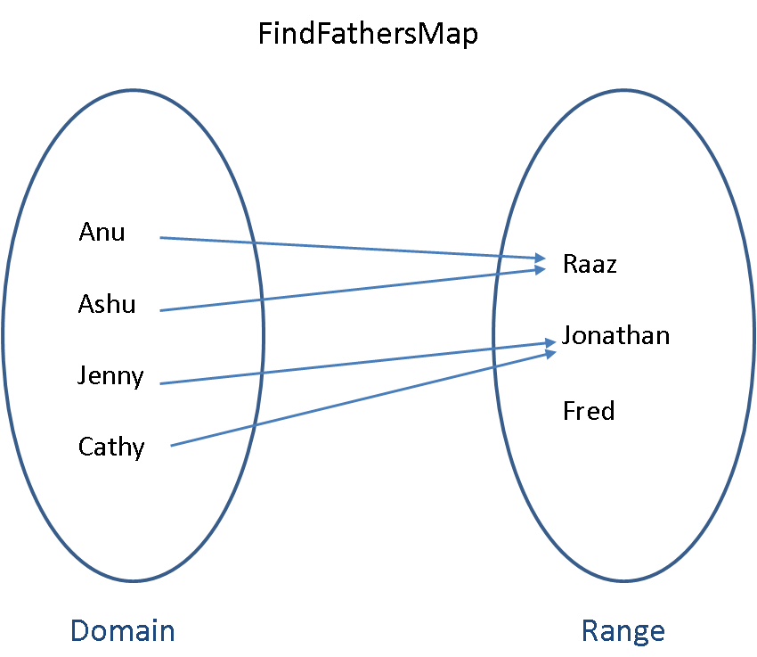
The notation for this mapping would be:
$$FindFathersMap: Daughters \rightarrow Men$$The domain is the set:
$$Daughters = \{Anu, Ashu, Jenny, Cathy\}$$and the range or codomain is the set:
$$Men = \{Raaz, Jonathan, Fred\}.$$The element in the range that an element in the domain maps to is called the image of that domain element.
For example, $Raaz$ is the image of $Anu$ in the $FindFathersMap$. The notation for this is:
Note that what we have just written is a function, just like the more familiar format of
$$f(x) = y \ .$$In computer science lingo each element in the domain is called a key and the images in the range are called values. The map or function associates each key with a value.
The keys for the map are unique since the domain is a set, i.e., a collection of distinct elements. Lots of keys can map to the same image value ($Jenny$ and $Cathy$ have the same father, $Anu$ and $Ashu$ have the same father), but the idea is that we can uniquely identify the value we want if we know the key. This means that we can't have multiple identical keys. This makes sense when you look at how the map works. We use the map to find values from the key, as we did when we found $Anu$'s father above. If we had more than one $Anu$ in the set of keys, we could not uniquely identify the value that maps to the key $Anu$.
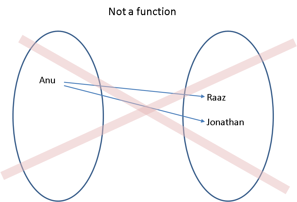
We do not allow maps (functions) where one element in the domain maps to more than one element in the range. In computer science lingo, each key can have only one value associated with it.
Formalising this, a function $f: \mathbb{X} \rightarrow \mathbb{Y}$ that maps each element $x \in \mathbb{X}$ to eaxctly one element $f(x) \in \mathbb{Y}$ is equivalent to the corresponding set of ordered pairs: $$\left\{(x, f(x)): x \in \mathbb{X}, f(x) \in \mathbb{Y}\right\} \ .$$
Here, $\left(x, f(x)\right)$ is an ordered pair (the familiar key-value pair in computer science).
The pre-image or inverse image of a function $f: \mathbb{X} \rightarrow \mathbb{Y}$ is $f^{[-1]}$.
The inverse image takes subsets in $\mathbb{Y}$ and returns subsets of $\mathbb{X}$.
The pre-image or inverse image of $y$ is $f^{[-1]}(y) = \left\{x \in \mathbb{X} : f(x) = y \right\} \subset \mathbb{X}$.
More generally, for any $B \subset \mathbb{Y}$:
$f^{[-1]}(B) = \{x \in \mathbb{X}: f(x) \in B \}$
For example, for our FindFathersMap,
- $FindFathersMap^{[-1]}(Raaz) = \{Anu, Ashu\}$ and
- $FindFathersMap^{[-1]}(Jonathan) = \{Jenny, Cathy\}$.
Now lets take a more mathematical looking function $f(x) = x^2$.
Version 1 of this function is going to have a finite domain (only five elements).
The domain is the set $\{-2, -1, 0, 1, 2\}$ and the range is the set $\{0, 1, 2, 3, 4\}$.
The mapping for version 1 is $$f(x) = x^2\,:\,\{-2, -1, 0, 1, 2\} \rightarrow \{0, 1, 2, 3, 4\} \ .$$
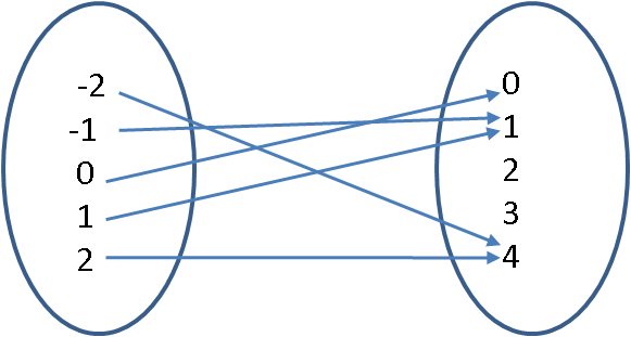
We can also represent this mapping as the set of ordered pairs $\{(-2,4), (-1,1), (0,0), (1,1), (2,4)\}$.
Note that the values 2 and 3 in the range have no pre-image in the domain. This is okay because not every element in the range needs to be mapped.
Having a domain with only five elements in it is a bit restrictive: how about an infinite domain?
Version 2
$$f(x) = x^2\,:\,\{\ldots, -2, -1, 0, 1, 2, \ldots\} \rightarrow \{0, 1, 2, 3, 4, \ldots\}$$
As ordered pairs, we now have $\{\ldots, (-2,4), (-1,1), (0,0), (1,1), (2,4), \ldots\}$, but it is impossible to write them all down since there are infinitely many elements in the domain.
What if we wanted to use the function for the whole of $\mathbb{R}$, the real line?
Version 3
$$f(x) = x^2 : \mathbb{R} \rightarrow \mathbb{R} \ . $$
def showURL(url, ht=500):
    """Return an IFrame of the url to show in notebook with height ht"""
    from IPython.display import IFrame
    return IFrame(url, width='95%', height=ht)
showURL('https://en.wikipedia.org/wiki/Function_(mathematics)#Introduction_and_examples',400)
Mathematical notation for functions
There are many notations for functions and it is a good idea to familiarize ourselves with some of them via examples. Scroll down the url function notation to become familiar with the following notations:
- $f: \mathbb{X} \to \mathbb{Y}$ or $\mathbb{X} \overset{f}{\to} \mathbb{Y}$ means $f$ is a function from $\mathbb{X}$ to $\mathbb{Y}$
- and $y=f(x)$ means $y \in \mathbb{Y}$ is equal to $f(x)$, the image of the function evaluated at $x \in \mathbb{X}$
Another convenient notation for a function is maps to denoted by $\mapsto$. For example, we can know the domain and range of a function and how it maps an argument to its image as follows:
- $f: \mathbb{N} \to \mathbb{Z}$ can be read as
- "$f$ is a function from $\mathbb{N}$ (the set of natural numbers) to $\mathbb{Z}$ (the set of integers)" or
- "$f$ is a $\mathbb{Z}$-valued function of an $\mathbb{N}$-valued variable"
- $x \mapsto 4-x$ can be read as "$x$ maps to $4-x$"
showURL("https://en.wikipedia.org/wiki/Function_(mathematics)#Notation",300)
In a computer, maps or functions are encoded as (i) sets of ordered pairs or as (ii) procedures.
Example 1: Encoding a function or map as a set of ordered pairs
In SageMath we can encode a map as a set of ordered pairs as follows.
findFathersMap = {'Jenny': 'Jonathan', 'Cathy': 'Jonathan', 'Anu': 'Raaz', 'Ashu': 'Raaz'}
findFathersMap
type(findFathersMap) # find the type of findFathersMap
findFathersMap is a Python/SageMath built-in datatype called dict which is short for dictionary. We will see dictionaries in more detail soon (or if you are imaptient see dict Python docs). For now, we are taking a mathematical view and learning to implement functions or maps as a set of ordered pairs.
Given a key (child) we can use the map to find the father.
findFathersMap['Anu']
print "The father of Anu is", findFathersMap['Anu'] # we can use a print statement to make it flow
We could also encode our inverse map of the findFathersMap as findDaughtersMap. We map from one father key (e.g. Raaz) to multiple values for daughters (for Raaz, it is Anu and Ashu).
findDaughtersMap = {'Jonathan': ['Jenny', 'Cathy'], 'Raaz': ['Anu', 'Ashu']}

# don't worry about the way we have done the printing below, just check the output makes sense to you!
for fatherKey in findDaughtersMap:
    print fatherKey, "has daughters:"
    for child in findDaughtersMap[fatherKey]:
        print '\t',child
We can also use a map for a numerical function $$y(x) = x^2 + 2: \{-2 ,-1 ,0, 1 ,2\} \to \{2, 3, 4, 5, 6\}$$ by encoding this function as a set of ordered pairs $$\{ (-2,6), (-1,3), (0,2), (1,3), (2,6)\}$$ in SageMath as follows.
myFunctionMap = {-2: 6, -1: 3,  0: 2, 1: 3, 2: 6}
myFunctionMap
Looking up the value or image of the keys in our domain $\{-2,-1,0,1,2\}$ works. Note the KeyError message when the key is outside the domain.
myFunctionMap[-2] # this return the value or image of the argument or key -2
myFunctionMap[-20] # KeyError: -20 since -20 is not in {-2,-1,0,1,2}
Example 2: Encoding function as a procedure
But it is clearly not a good way to try to specify a function mapping that can deal with lots of different $x$'s: in fact it would be impossible to try to specify a mapping like this if we want the domain of the function to have infinitely many elements (for example, if the domain is the set of all integers, or all rational numbers, or a segment of the real line, for example $f(x) = x^2 + 2 : \mathbb{R} \rightarrow \mathbb{R}$).
Instead, in SAGE we can just define our own function as a procedure that can evaluate our image value "on-the-fly" for any $x$ we want. We'll be doing more on functions in later labs so for the moment just think about how defining the function can be seen as a much more flexible way of specifying a mapping from the arguments in the domain of the function to values or images in its range.
The basics steps in encoding a function as a procedure in SageMath/Python:
- The function named
myFuncwe want to define for $x \mapsto x^2+2$ is preceeded by the keyworddeffor definition. - The function name
myFuncis succeeded by any input argument(s) to it within a pair of parentheses, for e.g.,(x)in this case since there is only one argument, namelyx. - After we have defined the function by its name
myFuncfollowed by its input argument(x)we end the line with a colon:before continuing to the next line. - Now, we are ready to write the body of the function. It is a customary to leave 4 white spaces. The number of spaces before a line or the indentation is used to delineate a block of code in SageMath/Python.
- It is a matter of courteous programming practice to enclose the Docstring, i.e., comments on what the function does, inside triple quotes. The Docstring is returned when we ask SageMath for help on the function.
- Finally, we output the image of our function with the keyword
returnand the expressionx^2+2.
def myFunc(x):                                 # starting the definition
    '''A function to return x^2 + 2'''         # the docstring
    return x^2+2                               # the function body (only one line in this example
myFunc?
When you evaluate the above cell you should see something like this:
Signature:      myFunc(x)
Docstring:      A function to return x^2 + 2
Init docstring: x.__init__(...) initializes x; see help(type(x)) for signature
File:           ~/all/git/scalable-data-science/_360-in-525/2018/04/jp/<ipython-input-18-ac2a17246c36>
Type: functionmyFunc(0.1) # use the function to calculate 0.1^2 + 2 with argument as a mpfr_real Literal
YouTry
When you evaluate the cell below, SageMath will complain about an IndentationError that you can easily fix.
def myFunc(x):
    '''A function to return x^2 + 2'''
     return x^2+2
The command to plot is pretty simple. The four arguments to plot are the function to be plotted, the input argument that is varying along the x-axis, the lower-bound and upper-bound of the input argument.
plot(myFunc(x),x, -20, 20)
?plot # for help hit the DocString of the function
We can get a bit more control of the figure size (and other aspects) by first assigning the plot to a variable and using the show method as follows.
myPlot = plot(myFunc(x),x, -20, 20)
myPlot.show(figsize=[6,3])

type(myPlot)
myPlot.show?
The simple plot command hides what is going on under the hood. Before we understand the fundamentals of plotting, let us get a better appreciation for the ordered pairs $(x,f(x))$ that make up the curve in this plot.
We can use SageMath to plot functions and add a way for you to interact with the plot. When you have evaluated this cell you'll see a plot of our function between $x=-20$ and $x=20$. The point on the curve where $x=3$ is indicated in red. You can alter the position of this point by putting a new value into the box at the top of the display (you can put in real number, eg 4.45, but if your number is outside the range -20 to 20 it won't be shown. Just try changing the value of x to plot as a point on the curve and don't worry about the way the code looks - you aren't expected to do this yourselves (at least not yet).
# Don't worry about this code and just interact with its output cell by changing the value in the box labelled x
@interact
def _(my_x=input_box(3, width=10, label="$x$")):
    myPt = (my_x, myFunc(my_x))
    myLabel = "(%.1f, %.1f)" % myPt
    p = plot(myFunc, (x,-20,20))
    if (my_x >= -20 and my_x <= 20):
        p += point(myPt,rgbcolor='red', pointsize=20)
        p += text(myLabel, (my_x+4,myFunc(my_x)), rgbcolor='red')
    p.show(figsize=[6,3])
A bit under plot's hood
The function you are viewing above from the plot command is actually just interpolated by a whole lot of points connected by lines!
To keep things more real let's expose the plot for what it really is next by only plotting a few points.
# plot 5 randomized points and leave them hanging
plot(myFunc,(-2,2), plot_points=5,marker='.',linestyle='', randomize=True, adaptive_recursion=0, figsize=[6,3])

# plot 5 randomized points and join them
plot(myFunc,(-2,2), plot_points=5,marker='.',linestyle='-', randomize=True, adaptive_recursion=0, figsize=[6,3])

# plot 100 randomized points and join them - now it looks continuous, doesn't it?
plot(myFunc,(-2,2), plot_points=100, marker='.',linestyle='-', randomize=True, adaptive_recursion=0, figsize=[6,3])

# plot 100 randomized points and join them without marker for points - now it looks like default plot, doesn't it?
plot(myFunc,(-2,2), plot_points=100, marker='',linestyle='-', randomize=True, adaptive_recursion=0, figsize=[6,3])

We will play with point, lines and other such objects in the sequel. For now, just remember that what you see is sometimes not what is under the hood.
You try
Define a more complicated function with four input arguments next. The rules for defining such a function are as before with the additional caveat of declaring all four input arguments inside the pair of parenthesis following the name of the function. In the cell below you will have to uncomment one line and then evaluate the cell to define the function (remember that comments begin with the # character).
# Here is a quadratic function of x with three additional parameters a,b,c
def myQuadFunc(a,b,c,x):
    '''A function to return a*x^2 + b*x + c'''
    return a*x^2 + b*x + c
Now try writing an expression to find out what myQuadFunc is for some values of x and coefficients a=1, b=0, c=2.
We have put the expression that uses these coefficients and x=10 into the cell below for you.
Can you see how Sage interprets the expression using the order in which we specified a, b, c, x in the definition above?
Try changing the expression to evaluate the function with same coefficients (a, b, c) but different values of x.
myQuadFunc(1, 0, 2, 10) # a = 1, b = 0, c = 2, x = 10
# we can make the same plot as before by letting a=1, b=0, c=2
plot(myQuadFunc(1,0,2,x),x, -20, 20, figsize=[6,3])

Example 3: Polymorphism and Type Errors
You can call the same function myFunc with different types and the operations in the body of the function, such a s power (^) and addition (+), will be automatically evaluated for the input type. This can be quite convenient!
When code is written without mention of any specific type and thus can be used transparently with any number of new types we are experiencing the concept of polymorphism (parametric plymorphism or generic programming).
myFunc(float(0.1)) # use the function to calculate 0.1^2 + 2 with argument as a Python float
myFunc(1/10) # use the function to calculate 0.1^2 + 2 with argument as a Sage Rational
myFunc(2) # use the function to calculate 0.1^2 + 2 with argument as a Sage Integer
myFunc(int(2)) # use the function to calculate 0.1^2 + 2 with argument as a Sage Rational
myFunc('hello') # calling myFunc on an input string argument results in a TypeError
We should see something like:
TypeError: unsupported operand parent(s) for +: '<type 'str'>' and 'Integer Ring'This is because in the body of myFunc(x) we have x^2+2 where x^2 is added to 2 using thr + operator, where 2 is a SageMath type Integer. And when we pass in the string hello for x by evaluating myFunc('hello') we are running into the mentioned TypeError of unsupported operand parents for +.
Interestingly, integer power of a string using the ^ operator is well defined as illustrated for hello below!
'hello'^2 # or 'hello'^2 = 'hellohello', i.e., 'hello' concatenated with itself two times
'hi'^3 # or 'hi'^3 = 'hihihi', i.e., 'hi' concatenated with itself three times
Also, addition of two string is also defined as concatenation:
'hello'+'hey'
Just to illustrate this, we next write a function named myFunc2 that returns x^2+x and will work for any input argument for which the operations of ^2 and + are well-defined for their operand parent types.
def myFunc2(x):
    '''square x and add x to it'''
    return x^2+x
myFunc2(0.1)
myFunc2('hi') # 'hi'^2 + 'hi' = 'hihi'+'hi' = 'hihihi'
Remark: such parametric polymorphism can be convenient but it can also have unintended consequences when you run the program. So be cautious!
Example 4: Mathematical functions
Many familiar mathematical functions such as $\sin$, $\cos$, $\log$, $\exp$ are also available directly in SageMath as built-in functions. They can be evaluated using parenthesis (brackets) as follows:
cos(0)
sin(0)
sin(pi)
print 'sin(pi) prints as', sin(pi)
# understand the output of each line and the symbolic/numeric expressions being evaluated and printed
print 'cos(1/2) prints as', cos(1/2)
print 'cos(1/2).n(digits=5) prints as', cos(1/2).n(digits=5)
print 'float(cos(1/2)) prints as', float(cos(1/2))
print 'cos(0.5) prints as', cos(0.5)

print 'exp(2*pi*e) prints as', exp(2*pi*e)

print 'log(10) prints as', log(10)
print 'log(10).n(digits=5) prints as', log(10).n(digits=5)
print 'float(log(10)) prints as', float(log(10))
print 'log(10.0) prints as', log(10.0)
You try
You can find out what built-in functions are available for a particular variable by typing the variable name followed by a . and then pressing the TAB key.
x=-2
x. # place the cursor after the . and press Tab
Try the abs function that evaluates the absolute value of x that is one of the methods available for x.
Here are two ways of calling abs method for x.
x.abs() #
abs(x)
Remember to ask for help!
If you want to know what a built-in function does, type the function name prepended by a '?'.
?abs
Collections in Sage
We have already talked about the SageMath and Python number types and a little about the string type. You have also met sets in SageMath with a brief mention of lists. A set and list in Sage are, loosely speaking, examples of collection types. Collections are a useful idea: grouping or collecting together some data (or variables) so that we can refer to it and use it collectively.
SageMath provides quite a few collections. One that we will meet very often is the list, a built-in sequence type in Python like the strings we have already seen. See Python tutorial for built-in data structures.
Example 1: Lists
Technically, a list in SageMath/Python is a sequence type. This basically means that the order of the things in the list is imporant and we can use concepts related to ordering when we work with a list. More specifically, a list is a mutable sequence type. This just means that you can change or mutate the contents of the list.
Don't worry about these details (unless you are interested in them of course and follow links below), but for now just look at the worksheet cells below to see how useful and flexible lists are.
When you want a list in SageMath you put the things in the list inside [ ] called square brackets. You can put almost anything in a list (including having lists of lists, as we'll see later).
L1 = []     # an empty list
L1          # display L1
L2 = ['orange', 'apple', 'lemon']   # a list of strings - remember that strings are within quote marks
L2                                  # display L2
L2.append('banana')                 # append something to the end of a list
L2                                  # display L2
L3 = [10, 11, 12 ,13] # a list of integers
type(L3) # type of L3 is
There are various functions and methods we can use with lists. For a more exhaustive dive see Python standard library docs specifically for the methods on lists that are:
In the interest of time, we are going to only familiarize ourselves with the immediately useful methods and learn new ones as we need them.
A very useful one is len, which gives us the length of the list, i.e., the number of elements in the list.
len(L3)
What about getting at the elements in a list once we have put them in? This is done by indexing into the list, or list indexing . Slightly confusingly, once you have a list, you index into it by using the [ ] brackets again.
L3[0] # the first position in the list is
Note that in SageMath the first position in the list is at position 0, or index [0] not at index [1]. In the list L3, which has 4 elements (len(L3) = 4), the indices are [0], [1], [2] and [3]. In the cell below you can check what you get when you ask for the element at the fourth position in the list (i.e., index [3] since the indexes start from [0]).
L3[3]
You will get an error message if the index you use is out of range (which means that you are trying to refer to something outside the range of the list). SageMath/Python "knows" that the list only has 4 elements, so asking for the element in the fifth position (index [4]) makes no sense and you get an IndexError: list out of range.
L3[4]
We can also get at more than one element in the list with the indexing operator [ ], by using : to indicate all elements from a position to another position. This slicing of a list is hard to explain in words but easy to see in action.
L3[0:2] # elements in positions 0 to 2 in list L3 are
If you leave out the starting and ending positions and just use [:] you'll get the whole list. This is useful for making copies of whole lists.
L4 = L3[:]
L4             # disclose L4
SageMath also provides some helpful ways to make lists quickly. The one you'll use most often is range. Used in its most simple form, range(n) gives you a list of n integers from 0 to n-1.
L5 = range(10)                      # a quick way to make a list of 10 numbers starting from 0
L5
Note that the numbers you get start from 0 and the last one is 9.
You'll see that we can get even cleverer and use range to get a list that starts and stops at specified numbers with a specified step size between the numbers. Let's try this to get numbers in steps of 5 from 100 to 145, in the cell below.
L6 = range(100, 150, 5)   # get a list with a specified start, stop and step
L6
Notice that again we don't go right up to the "stop" number (200) but to the last one below it taking into account our step size (5), ie 145.
When we just asked for range(10) SageMath assumed a default start of 0 and a default step of 1. Thus, range(10) is equivalent to range(0, 10, 1).
YouTry
Start of this YouTry
Find out more about list and range by evaluating the cells below and looking at the Python docs (see links above) or just via DocStrings.
?range
help(list.append) # or use help for brief DocStrings
Make yourself a list with some elements in it; you can choose how many elements to have and what type they are.
Assign the list to a variable named myList.
myList = [ REPLACE_THIS_WITH_ELEMENTS_OF_LIST ]
Add a new element to myList using the .append method.
Use the nice way of copying we showed you above (remember, [:]) to copy everything in myList to a new list called myNewList. Use the len function to check the length of your new list.
myNewList = myList[ REPLACE_THIS_WITH_THE_RIGHT_CHARACTER ]
len(myNewList)
Use the indexing operator [ ] to find out what the first element in myList is (remember that the index of the first element will be 0).
myList[ FILL_IN_HERE ]
Use the indexing opertor [ ] to change the first element in myNewList to some different value.
myNewList[0] = FILL_IN_HERE
Disclose the original list, myList, to check that nothing in that has changed.
print myList
print myNewList
Use range to make a list of the integer numbers between 4 and 16, going up in steps of 4. Assign this list to a variable named rangeList.
rangeList = range( FILL_IN_HERE )
Disclose your list rangeList to check the contents. You should have the values 4, 8, 12, 16. If you don't, check what you asked for in the cell above and fix it up to give the values that you wanted.
rangeList
END of YouTry
Example 2: Tuples
A tuple is another built-in sequence type in Python like lists and strings. The values in a tuple are enclosed in curved parentheses ( ) and the values are separated by commas.
myTuple1 = (1, 2) # assign the tuple (1,2) to variable nemed muTuple1
myTuple1
type(myTuple1)
myTuple2 = (10, 11, 13)
myTuple2
Tuples are immutable. In programming, an 'immutable' object is an object whose state cannot be modified after it has been created (Etymology: 'mutable comes from the Latin verb mutare, or 'to change' -- the same root we get 'mutate' from. So in-mutable, or immutable, means not capable of or susceptible to change). This means that although we can access the element at a particular position in a tuple by indexing ...
myTuple1[0] # disclose what is in the first position in the tuple
... we can't change what is in that particular position in the tuple.
myTuple1[0] = 10 # try to assign a different value to the first position in the tuple
myTuple1[0] # the first element in the tuple is immutably 1
Useful things you can do with tuples
Sage has a very useful zip function. Zip can be used to 'zip' sequences together, making a list of tuples out of the values at corresponding index positions in each list. Consider a simple example: Note that in general zip works with sequences, so it can be used to zip tuples as well as lists.
zip(['x', 'y', 'z'], [1, 2, 3])
Example 3: Sets
We already created and assigned sets and operated with them. Set/set are another SageMath/Python collection. Remember that in a set, each element has to be unique. We can specify a set directly or make one out of a list.
L6 = range(100, 150, 5)  # make sure we have a list L6
S = set(L6)     # make the set S from the list L6
S             # display the set s
Sets are unordered collections. This makes sense when we think about what we know about sets: what matters about a set is the unique elements in it.
The set $\{1, 2, 3\}$ is the same as the set $\{1, 3, 2\}$ is the same as the set $\{2, 3, 1\}$, etc.
This means that it makes no sense to ask SageMath what's at some particular position in a set as we could with lists. Lists are sequnces and order matters. Sets are unordered - order makes no sense for a set.
We cannot use the indexing operator [ ] with a set.
S[0] # will give an error message 'TypeError: 'set' object does not support indexing'
S. # put the cursor after the . and hit Tab to see all the methods available on Python set
SS = Set(L6) # this is a SageMath set with upper-case Set
SS. # put the cursor after the . and hit Tab to see all the extra methods available on SageMath Set
Example 4: Dictionaries
When we created our maps or functions at the start of this worksheet, we actually used dictionaries: A SageMath/Python dictionary gives you a way of mapping from a key to a value. As we said earlier, the keys have to be unique (only one of each key) but more than one key can map to the same value. Remember the FindFathersMap? It is actually a Python dictionary or simply dict.
Although, we used the syntax for dictionaries to conceptually reinforce functions and maps, we revisit them here and contrast them with the other collections we have already seen like lists and sets.
findFathersMap = {'Jenny': 'Jonathan', 'Cathy': 'Jonathan', 'Anu': 'Raaz', 'Ashu': 'Raaz'}
findFathersMap
type(findFathersMap)
When we make a dictionary, we tell SageMath that it is a dictionary by using the curly brackets { } and by giving each key value pair in the format key: value.
A dictionary has something like the indexing operator we used for lists, but instead of specifying the position we want (like [0]) we specify the key we want, and SageMath returns the value that key maps to.
findFathersMap['Anu'] # who is Anu's father
Manipulating a dict
In the cell below we have the start of a simple dictionary for phone numbers.
myPhoneDict = {'Ben': 8888, 'Raaz': 3333}
myPhoneDict     # disclose the contents of the dictionary
In the cell below let us add susy with phone number 78987 to our dictionary.
myPhoneDict['susy']=78987
myPhoneDict # disclose the current contents of our dict
zip-ping of tuples gives us a quick way to make a dictionary if we have separate lists or tuples which contain our keys and values. Note that the ordering in the key and value sequences has to be consistent -- the first key will be mapped to the first value, etc., etc.
myKeys = ('Ben', 'Raaz', 'susy')
myValues = (888, 333, 78987)
myPhoneDictByZip = dict(zip(myKeys, myValues))
myPhoneDictByZip
You try
Try adding to what we have to put in two more people, Fred, whose phone number is 1234, and Mary whose phone number is 7777.
Remember that for SageMath, the names Fred and Mary are strings and you must put them in quote marks, like the names that are already there.
myPhoneDictByZip['Fred']=1234
myPhoneDictByZip['Mary']=7777
myPhoneDictByZip
Now try asking SageMath for Ben's phone number (ie, the phone number value associated with the key Ben).
myPhoneDictByZip['Ben']
There are also some useful methods of dictionaries that allow you to 'dissect' the dictionary and extract just the keys or just the values.
myPhoneDictByZip.keys()
myPhoneDictByZip.values()
And there is also an .items() method that gives you back your your (key, value) pairs again. You will see that is it a list of tuples.
myPhoneDictByZip.items()
Probability
(This is a partial type-setting of the notes scribed on the black board.)
The origins of probability can be traced back to the 17th century. It arose out of the study of gambling and games of chance. Many well-known names associated with probability worked on problems to do with gambling: people like Bernoulli and Pascal did quite a lot of work in this area ... even Newton was persuaded to set down some of his thoughts about a game involving dice (in a letter to a Samuel Pepys).
Dive into the main wikipedia article here for more details. Here, we will take the shortest mathemtical path to understanding probability.
Probability has a language of its own. We are going to introduce you to some of the essential terms:
An experiment is an activity or procedure that produces distinct or well-defined outcomes. The set of such outcomes is called the sample space of the experiment. The sample space is usually denoted with the symbol $\Omega$. Lets look at some examples of experiments.
Roll a dice experiment
If our experiment is to roll a dice wth faces painted $red$, $green$, $yellow$, $pink$, $blue$ and $black$ and find what colour the top face is at the end of each roll, then the sample space $\Omega = \{red, green, yellow, pink, blue, black\}$.
Flip a coin experiment
If our experiment is to flip a coin where the two faces of the coin can be identified as 'heads' ($H$) and 'tails' ($T$), and we are interested in what face lands uppermost, then the sample space is $\Omega = \{H, T\}$.
Draw a fruit from a fruit bowl
Suppose we have a well-mixed fruit bowl that contains:
- 2 oranges
- 3 apples
- 1 lemon
If our experiment is to take a single fruit from the bowl and the outcome is the type of fruit we take then what is the sample space for this experiment?
Recall that the sample space is the set of all possible outcomes of the experiment. If we take a single fruit we could get only one of the three fruits in each draw: an orange, or an apple or a lemon. The sample space $\Omega = \{orange, apple, lemon\}$.
An event is a subset of the sample space. For example, we could take the event $\{orange, lemon\} \subset \Omega$ in the fruit bowl experiment.
Probability maps a set of events to a set of numbers in a certain axiomatic manner. Abstractly, probability is a function that assigns numbers in the range 0 to 1 to events
$$P : \text{set of events } \rightarrow [0,1]$$which satisfies the following axioms:
- For any event $A$, $ 0 \le P(A) \le 1$.
- If $\Omega$ is the sample space, $P(\Omega) = 1$.
- If $A$ and $B$ are disjoint (i.e., $A \cap B = \emptyset$), then $P(A \cup B) = P(A) + P(B)$.
- If $A_1, A_2, \ldots$ is an infinite sequence of pair-wise disjoint events (i.e., $A_i \cap A_j = \emptyset$ when $i \ne j$), then $$ \begin{array}{lcl} \underbrace{P\left(\bigcup_{i=1}^{\infty}A_i\right)} &=& \underbrace{\sum_{i=1}^{\infty}P\left(A_i\right)} \\ A_1 \cup A_2 \cup A_3 \dots &=& P(A_1) + P(A_2) + P(A_3) + \ldots \end{array} $$
These axioms or assumptions are motivated by the frequency interpretation of probability. The frequency interpretation of probability says that if we repeat an experiment a very large number of times then the fraction of times that the event $A$ occurs will be close to $P(A)$.
More precisely,
$$ \begin{array}{llcl} \mbox{let } & N(A, n) & = & \mbox{ the number of times } A \mbox{ occurs in the first } n \mbox{ trials,} \\ \mbox{then } & P(A) & = & \lim_{n \rightarrow \infty} \frac{N(A, n)}{n} \end{array} $$To think about this, consider what $\lim_{n \rightarrow \infty} \frac{N(A, n)}{n}$ is:
$$ \begin{array}{c} \frac{N(A, 1)}{1},\, \frac{N(A, 2)}{2},\,\frac{N(A, 3)}{3},\,\ldots \mbox{where is this fraction going?} \end{array} $$Let's look at axioms 1, 2, and 3 above more closely.
For any event $A$, $ 0 \le P(A) \le 1$. Well, clearly $0 \le \frac{N(A, n)}{n} \le 1$.
If $\Omega$ is the sample space, $P(\Omega) = 1$. This essentially says "something must happen". $P(\Omega) = \frac{N(\Omega, n)}{n} = \frac{n}{n} = 1$.
If $A$ and $B$ are disjoint (i.e., $A \cap B = \emptyset$), then $N(A \cup B, n) = N(A, n) + N(B, n)$ since $A \cup B$ occurs if either $A$ or $B$ occurs but we know that it is impossible for both $A$ and $B$ to happen (the intersection is the empty set). This extends to infinitely many disjoint events.
Axiom 4 is a bit more controversial, but here we assume it as part of our axiomatic definition of probability (without it the maths is much harder!).
Lets do some probability examples.
Example 1: Tossing a fair coin
The sample space and probabilties of this experiment are:
$$\Omega = \{H, T\}, \ \text{and} \ P(\{H\}) = P(\{T\}) = \frac{1}{2} \ .$$We can represent our probability as the following function:
- $P : \{ \{H\} , \{T\}, \{H,T\}, \{\} \} \to \{0,\frac{1}{2},1\}$,
- with $P(\{H\})=\frac{1}{2}$, $P(\{T\})=\frac{1}{2}$, $P(\{H,T\})=1$ and $P(\{\})=0$.
notational convenience: The outcomes which are the elements in the the sample space are denoted without set brackets, for example: $P(\{H\})$ is denoted by $P(H)$ for brevity.
Check that all our axioms are satisfied:
- yes! because: $0 \le P(H) = P(T) = \frac{1}{2} \le 1$ and $0 \le P(\Omega) = 1 \le 1$.
- yes! becasue: $P(\Omega) = P(\{H, T\} = P(\{H\}) + P(\{T\}) = \frac{1}{2} + \frac{1}{2} = 1$.
- yes!, because: $P(\{H, T\} = P(\{H\}) + P(\{T\})$.
Example 2: Tossing an unfair coin
$\Omega = \{H, T\}$, $P(H) =\frac{3}{4}$, $P(T) = \frac{1}{4}$. So the coin lands heads 3 out of 4 times and lands tails only 1 out of 4 times.
Check that all our axioms are satisfied:
- $0 \le P(H) = \frac{3}{4} \le 1$, $0 \le P(T) = \frac{1}{4} \le 1$ and $0 \le P(\Omega) = 1 \le 1$.
- $P(\Omega) = P(\{H, T\} = P(\{H\}) + P(\{T\}) = \frac{3}{4} + \frac{1}{4} = 1$.
- $P(\{H, T\} = P(\{H\}) + P(\{T\})$.
Yes, all three axioms are satisfied by the probabiliy for this unfair coin experiment too.
Example 2': Tossing an unfair coin $m$ times to construct a random graph
From Wikipedia:
In the mathematical field of graph theory, the Erdős–Rényi model is either of two closely related models for generating random graphs. They are named after mathematicians Paul Erdős and Alfréd Rényi, who first introduced one of the models in 1959,12 while Edgar Gilbert introduced the other model contemporaneously and independently of Erdős and Rényi.3
In the model of Erdős and Rényi, all graphs on a fixed vertex set with a fixed number of edges are equally likely; in the model introduced by Gilbert, each edge has a fixed probability of being present or absent, independently of the other edges.
Draw the construction on a graph with $n$ vertices and $m$ edges.
What is exactly a Graph?
<br><br><br ><br >
showURL("https://en.wikipedia.org/wiki/Erd%C5%91s%E2%80%93R%C3%A9nyi_model",400)
Example 3: New Zealand Lotto
In New Zealand Lotto, the balls drawn are numbered 1 to 40. The number on a ball is an outcome.
$\Omega = \{1, 2, \ldots,40\}$, $P(\omega) = \frac{1}{40}$ for each $\omega \in \Omega$ (i.e., $P(1) = P(2) = \ldots = P(40) = \frac{1}{40}$)
Now, consider the event that the first ball is even? What is the probability of this event, $P(\{2, 4, 6, \ldots, 38, 40\})$?
$$ \begin{array}{lcll} P(\{2, 4, \ldots, 38, 40\}) & = & P \left( \{2\} \cup \{4\} \cup \cdots \cup \{38\} \cup \{40\} \right) & \mbox{(defn. of set union)}\\ & = & P( \{2\}) +P( \{4\}) + \cdots + P(\{38\}) + P( \{40\}) & \mbox{(extn. Axiom 3)} \\ & = & \sum_{i \in \{2, 4, \ldots, 40\}} P(\{i\}) & \\ & = & 20 \times \frac{1}{40} & \\ & = & \frac{1}{2} & \end{array} $$Similarly for the probability of an odd ball:
$$ \begin{array}{lcl} P(\{1, 3, 5, \ldots, 37, 39\}) & = & P \left( \{1\} \cup \{3\} \cup \cdots \cup \{37\} \cup \{39\} \right)\\ & = & P(\{1\}) +P( \{3\}) + \cdots + P(\{37\}) + P( \{39\})\\ & = & \sum_{i \in \{1, 3, \ldots, 37, 39\}} P(\{i\}) \\ & = & 20 \times \frac{1}{40} \\ & = & \frac{1}{2} \end{array} $$Aside: The set of all possible subsets of $\Omega$ is called the power set and is denoted by $2^{\Omega}$. The power set contains all events of a sample space and is a natural domain for the probability function defined on a sample space with finitely many outcomes. We will see more on this later but if you are impatient see here.
Now, having introduced a number of definitions, we will derive some basic logical consequences, (i.e., properties) of probabilities (axiomatically defined).
Property 1
$P(A) = 1 - P(A^c)$, where $A^c = \Omega \setminus A$ is the complement of $A$.
Proof
$A \cap A^c = \emptyset$ and $A \cup A^c = \Omega$
Recall that axiom 3 says that if $A_1 \cap A_2 = \emptyset$ then $P(A_1 \cup A_2) = P(A_1) + P(A_2)$
So this implies that $P(A) + P(A^c) = P(\Omega) = 1$, by axiom 2 which says that $P(\Omega) = 1$
Subtracting $P(A^c)$ from both sides, we get $P(A) + P(A^c) - P(A^c) = 1 - P(A^c)$
Cancelling out the two $P(A^c)$ terms on the right hand side, we get $P(A) = 1 - P(A^c)$ .
For example, in the coin tossing experiment, $\Omega = \{H, T\}$
$$P(H) = 1 - P(H^c) = 1 - P(\Omega \setminus H) = 1 - P(T)$$Property 2
For any two events $A$, $B$,
$P(A \cup B) = P(A) + P(B) - P(A \cap B)$
Proof:
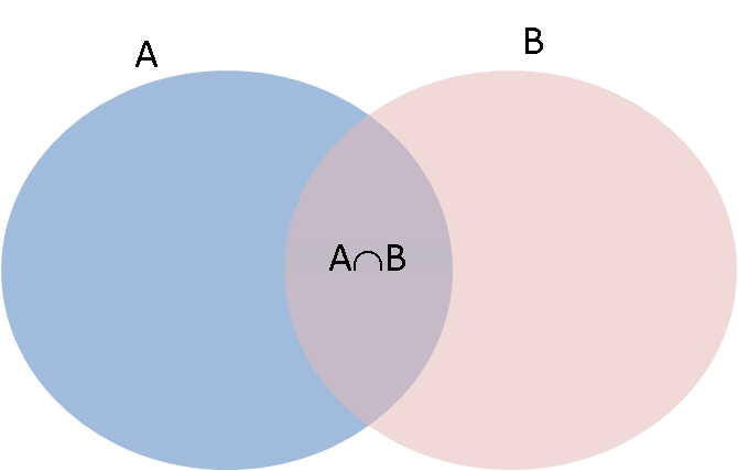
This is an informal proof using the picture above. If we just add the probabilities of $A$ and $B$ we will double count the probabilties of the outcomes which are in both $A$ and $B$. We adjust for this double counting by subtracting $P(A \cap B)$.
Note that if $A \cap B = \emptyset$ then $P(A \cap B) = 0$ and $P(A \cup B) = P(A) + P(B)$.
Computer Representations of Mathematical Concepts and Objects
So we have probabilities associated with events satisfying some axioms -- that sounds like a good use for a dictionary? That's basically what are going to use, but we 'wrap' up the dictionary in some extra code that does things like check that the probabilities add to 1, and that each element in the list of outcomes we have given is unique. If you are interested in programming, we have coded our own type, or class, called ProbyMap (it's given in the next cell, and you can simply evaluate it and ignore all the details completely!). Once the class is coded, we create a ProbyMap by providing the sample space and the probabilities. You don't have to worry about how the class is implemented, but note that you may often want to use the computer to create a computerised representation of a mathematical concept. Once the concept (a discrete probability map in our case) is implemenetd, then we can use the computer to automate the mundane tasks of large-scale computations.
SageMath already has some such implementations that are more sophisticated and general:
Here we will roll our own for pedagogical reasons.
# create a class for a probability map - if you are new to SageMath/Python just evaluate and skip this cell
# This was coded by Jenny Harlow

import copy
class ProbyMap(object):                # class definition
    'Probability map class'
    def __init__(self, sspace, probs): # constructor
        self.__probmap = {}  # default probmap is empty
        # make checks on the objects given as sspace and probs
        try:
            sspace_set = set(sspace) # check that we can make the sample space into a set
            assert len(sspace_set) == len(sspace) # and not lose any elements
            prob_list = list(probs) # and we can make the probs into a list
            probsum = sum(prob_list) # and we can sum the probs
            assert probsum == 1 # and the probs sum to 1
            assert len(prob_list) == len(sspace_set) # and there is proby for each event

            self.__probmap = dict(zip(list(sspace),prob_list))    # map from sspace to probs

        except TypeError, diag: # if there any problems with types
            init_error = 1
            print str(diag)

        except AssertionError:
            init_error = 1
            print "Check sample space and probabilities"


    def P(self, events):
        '''Return the probability of an event or set of events.

        events is set of events in the sample space to calculate the probability for.'''

        retvalue = 0
        try:
            events_set = set(events) # check we can make a set out of the events
            assert len(events_set) == len(events) # and not lose any events
            assert events_set <= set(self.__probmap.keys()) # events subset of sample space

            for ev in events:     # add each mapped probability to the return value
                retvalue += self.__probmap[ev]

        except TypeError, diag:
            print str(diag)

        except AssertionError:
            print "Check your events"

        return retvalue

    def __str__(self):                            # redefine printable string rep
        'Printable representation of the object.'
        num_keys = len(self.__probmap.keys())
        counter = 0
        retval = '{'
        for each_key in self.__probmap:
            counter += 1
            retval += str(each_key)
            retval += ': '
            retval += "%.3f" % self.__probmap[each_key]
            if counter < num_keys:
                retval += ', '
        retval += '}'

        return retval

    __repr__ = __str__

    def get_probmap(self):                        # get a deep copy of the proby map
        return copy.deepcopy(self.__probmap)      # getter cannot alter object's map

    probmap = property(get_probmap)               # allow read access via .probmap

    def get_ref_probmap(self):                    # get a reference to the real probmap
        return self.__probmap                     # getter can alter the object's map


    ref_probmap = property(get_ref_probmap)       # allow access via .ref_probmap

    @staticmethod
    def dictExp(big_map, small_map):
        '''Internal helper function for __pow__(...).

        Takes two proby map dictionaries and returns one mult by other.'''
        new_bl = {}
        for sle in small_map:
            for ble in big_map:
                new_key = str(ble) + ' ' + str (sle)
                new_bl[new_key] = big_map[ble]*small_map[sle]
        return new_bl

    def __pow__(self, x):
        '''probability map exponentiated.'''
        try:
            assert isinstance(x, Integer)
            pmap = copy.deepcopy(self.__probmap) # copy the probability map dictionary
            new_pmap = copy.deepcopy(self.__probmap) # and another copy
            for i in range(x-1):
                new_pmap = self.dictExp(new_pmap, pmap)

            return ProbyMap(new_pmap.keys(), new_pmap.values())

        except AssertionError:
            print "cannot raise to non-integer power"
            return None
Example 4: Experiments, outcomes, sample spaces, events, and the probability of events
Let's go back to the well-mixed fruit bowl experiment. The fruit bowl contains:
- 2 oranges
- 3 apples
- 1 lemon
The experiment is to take one piece of fruit from the bowl and the outcome is the type of fruit we get.
The sample space is $\Omega = \{orange, apple, lemon\}$
We can use the Sage list to create this sample space (a list is a bit easier to use than a set, but using a list means that we are responsible for making sure that each element contained in it is unique).
# sample space is the set of distinct type of fruits in the bowl
samplespace = ['orange', 'apple', 'lemon']
We can also use a list to specify what the probability of each outcome in the sample space is. The probabilities can be calculated by knowing how many fruits of each kind are there in the bowl. We say that the fruit bowl is 'well-stirred', which essentially means that when we pick a fruit it really is a 'random sample' from the bowl (for example, we have not carefully put all the apples on the top so that someone will almost certainly get an apple when they take a fruit). More on this later in the course! Note that the probabilities encoded by a list named probabilities are in the same order as the outcomes in the samplespace list.
# probabilities take into account the number of each type of fruit in the "well-stirred" fruit bowl
probabilities = [2/6, 3/6, 1/6]
probMapFruitbowl = ProbyMap(sspace = samplespace, probs=probabilities) # make our probability map
probMapFruitbowl         # disclose our probability map
We can use our probability map to find the probability of a single outcome like this:
# Find the probability of outcome 'lemon'
probMapFruitbowl.P(['lemon'])
We can also use our probability map to find the probability of an event (set of outcomes).
# Find the probability of the event {lemon, orange}
probMapFruitbowl.P(['lemon','orange'])
Basically, the probability map implemenetd by ProbyMap is essentially a map or dictionary with some additional bells and whistles.
Basically, the probability map is essentially a map or dictionary.
Next we will obtain the set of all events (the largest $\sigma$-algebra or $\sigma$-field in math lingo) from the outcomes in our sample space via the Subset function and find the probability of each event using our ProbyMap in a for loop.
# make the set of all possible events from the set of outcomes
setOfAllEvents = Subsets(samplespace)  # Subsets(A) returns the set of all subsets of A
list(setOfAllEvents)    # disclose the set of all events
We have not done loops yet, but we will soon. Just as a foretaste, here we use a for loop to print out the computed probabilities for each event in the setOfAllEvents.
# loop through the set of all events and print the computed probability
for event in setOfAllEvents:
    print "P(", event, ") = ", probMapFruitbowl.P(event)
YouTry
Try working through Example 6 below for yourself in the tutorial.
Example 5: Experiments with the English language
In English language text there are 26 letters in the alphabet. The relative frequencies with which each letter appears is tabulated below:
| E | 13.0% | H | 3.5% | W | 1.6% |
| T | 9.3% | L | 3.5% | V | 1.3% |
| N | 7.8% | C | 3.0% | B | 0.9% |
| R | 7.7% | F | 2.8% | X | 0.5% |
| O | 7.4% | P | 2.7% | K | 0.3% |
| I | 7.4% | U | 2.7% | Q | 0.3% |
| A | 7.3% | M | 2.5% | J | 0.2% |
| S | 6.3% | Y | 1.9% | Z | 0.1% |
| D | 4.4% | G | 1.6% |
Using these relative frequencies as probabilities we can create a probability map for the letters in the English alphabet. We start by defining the sample space and the probabilities.
alphaspace = ['A','B','C','D','E','F','G','H','I','J','K','L','M','N','O','P','Q',
              'R','S','T','U','V','W','X','Y','Z']
alphaRelFreqs = [73/1000,9/1000,30/1000,44/1000,130/1000,28/1000,16/1000,35/1000,74/1000,
                 2/1000,3/1000,35/1000, 25/1000,78/1000,74/1000,27/1000,3/1000,77/1000,63/1000,
                 93/1000,27/1000,13/1000,16/1000,5/1000,19/1000,1/1000]
Then we create the probability map, represented by a ProbyMap object.
probMapLetters = ProbyMap(sspace = alphaspace, probs=alphaRelFreqs) # make our probability map
probMapLetters         # disclose our probability map
Please do NOT try to list the set of all events of the 26 alphabet set: there are over 67 million events and the computer will probably crash! You can see how large a number we are talking about by evaluating the next cell which calculates $2^{26}$ for you.
2^26
Instead of asking for the probability of each event (over 67 million of them to exhaustively march through!) we define some events of interest, say the vowels in the alphabet or the set of letters that make up a name.
vowels = ['A', 'E', 'I', 'O', 'U']
And we can get the probability that a letter drawn from a 'well-stirred' jumble of English letters is a vowel.
probMapLetters.P(vowels)
We can make ourselves another set of letters and find probabilities for that too. In the cell below, we go straight from a string to a set. The reason that we can do this is that a string or str is in fact another collection; str is a sequence type just like list.
NameOfRaaz=set("RAAZESHSAINUDIIN")        # make a set from a string
NameOfRaaz                                # disclose the set NameOfRaaz you have built
probMapLetters.P(NameOfRaaz)
Try either adapting what we have above, or doing the same thing in some of cells below, to find the probabilities of other sets of letters yourself. For example, what is the probability of your name in the above sense?
The crucial point of the above exercise with our own implementation of a Python class for probability maps is to show how computers and mathematics can go hand in hand to quickly generalize operations over specific instances of a large class of mathematical notions (Example 4 and 5 for probability models on finite sample spaces in our case above).
A Coming Attraction!
Recall how we downloaded Pride and Prejudice and processed it as a String and break it by Chapters. This is at our disposal - all we need to do is copy-paste the right set of cells from earlier here to have the string from that Book by fetching live from the Guthenberg Project again.
Think about what algorithmic constructs and methods one will need to split each sentence by words it contains and count the number of each distinct word.
We will need to understand for loops, list comprehensions and anonymous functions, as well as methods on strings for splitting (which you can search by adding a . after a srt and hitting the Tab button to look through exixting methods), and more crucially the data-structure we just saw called the dictionary, as we will see shortly.