// Databricks notebook source exported at Tue, 28 Jun 2016 06:48:35 UTC
Scalable Data Science
prepared by Raazesh Sainudiin and Sivanand Sivaram
supported by  and
and

The html source url of this databricks notebook and its recorded Uji  :
:
#Topic Modeling with Latent Dirichlet Allocation
This is an augmentation of a notebook from Databricks Guide.
This notebook will provide a brief algorithm summary, links for further reading, and an example of how to use LDA for Topic Modeling.
##Algorithm Summary
- Task: Identify topics from a collection of text documents
- Input: Vectors of word counts
- Optimizers:
- EMLDAOptimizer using Expectation Maximization
- OnlineLDAOptimizer using Iterative Mini-Batch Sampling for Online Variational Bayes
Links
- Spark API docs
- MLlib Programming Guide
- ML Feature Extractors & Transformers
- Wikipedia: Latent Dirichlet Allocation
Readings for LDA
- A high-level introduction to the topic from Communications of the ACM
- A very good high-level humanities introduction to the topic (recommended by Chris Thomson in English Department at UC, Ilam):
Also read the methodological and more formal papers cited in the above links if you want to know more.
Let’s get a bird’s eye view of LDA from https://www.cs.princeton.edu/~blei/papers/Blei2012.pdf next.
- See pictures (hopefully you read the paper last night!)
- Algorithm of the generative model (this is unsupervised clustering)
- For a careful introduction to the topic see Section 27.3 and 27.4 (pages 950-970) pf Murphy’s Machine Learning: A Probabilistic Perspective, MIT Press, 2012.
- We will be quite application focussed or applied here!
//This allows easy embedding of publicly available information into any other notebook
//when viewing in git-book just ignore this block - you may have to manually chase the URL in frameIt("URL").
//Example usage:
// displayHTML(frameIt("https://en.wikipedia.org/wiki/Latent_Dirichlet_allocation#Topics_in_LDA",250))
def frameIt( u:String, h:Int ) : String = {
      """<iframe
 src=""""+ u+""""
 width="95%" height="""" + h + """"
 sandbox>
  <p>
    <a href="http://spark.apache.org/docs/latest/index.html">
      Fallback link for browsers that, unlikely, don't support frames
    </a>
  </p>
</iframe>"""
   }
displayHTML(frameIt("http://journalofdigitalhumanities.org/2-1/topic-modeling-and-digital-humanities-by-david-m-blei/",900))
displayHTML(frameIt("https://en.wikipedia.org/wiki/Latent_Dirichlet_allocation#Topics_in_LDA",250))
displayHTML(frameIt("https://en.wikipedia.org/wiki/Latent_Dirichlet_allocation#Model",600))
displayHTML(frameIt("https://en.wikipedia.org/wiki/Latent_Dirichlet_allocation#Mathematical_definition",910))
Probabilistic Topic Modeling Example
This is an outline of our Topic Modeling workflow. Feel free to jump to any subtopic to find out more.
- Step 0. Dataset Review
- Step 1. Downloading and Loading Data into DBFS
- (Step 1. only needs to be done once per shard - see details at the end of the notebook for Step 1.)
- Step 2. Loading the Data and Data Cleaning
- Step 3. Text Tokenization
- Step 4. Remove Stopwords
- Step 5. Vector of Token Counts
- Step 6. Create LDA model with Online Variational Bayes
- Step 7. Review Topics
- Step 8. Model Tuning - Refilter Stopwords
- Step 9. Create LDA model with Expectation Maximization
- Step 10. Visualize Results
Step 0. Dataset Review
In this example, we will use the mini 20 Newsgroups dataset, which is a random subset of the original 20 Newsgroups dataset. Each newsgroup is stored in a subdirectory, with each article stored as a separate file.
The following is the markdown file 20newsgroups.data.md of the original details on the dataset, obtained as follows:
$ wget -k http://kdd.ics.uci.edu/databases/20newsgroups/20newsgroups.data.html
--2016-04-07 10:31:51--  http://kdd.ics.uci.edu/databases/20newsgroups/20newsgroups.data.html
Resolving kdd.ics.uci.edu (kdd.ics.uci.edu)... 128.195.1.95
Connecting to kdd.ics.uci.edu (kdd.ics.uci.edu)|128.195.1.95|:80... connected.
HTTP request sent, awaiting response... 200 OK
Length: 4371 (4.3K) [text/html]
Saving to: '20newsgroups.data.html’

100%[======================================>] 4,371       --.-K/s   in 0s

2016-04-07 10:31:51 (195 MB/s) - '20newsgroups.data.html’ saved [4371/4371]

Converting 20newsgroups.data.html... nothing to do.
Converted 1 files in 0 seconds.

$ pandoc -f html -t markdown 20newsgroups.data.html > 20newsgroups.data.md
20 Newsgroups
Data Type
text
Abstract
This data set consists of 20000 messages taken from 20 newsgroups.
Sources
Original Owner and Donor
Tom Mitchell
School of Computer Science
Carnegie Mellon University
tom.mitchell@cmu.edu
Date Donated: September 9, 1999
Data Characteristics
One thousand Usenet articles were taken from each of the following 20 newsgroups.
    alt.atheism
    comp.graphics
    comp.os.ms-windows.misc
    comp.sys.ibm.pc.hardware
    comp.sys.mac.hardware
    comp.windows.x
    misc.forsale
    rec.autos
    rec.motorcycles
    rec.sport.baseball
    rec.sport.hockey
    sci.crypt
    sci.electronics
    sci.med
    sci.space
    soc.religion.christian
    talk.politics.guns
    talk.politics.mideast
    talk.politics.misc
    talk.religion.misc
Approximately 4% of the articles are crossposted. The articles are typical postings and thus have headers including subject lines, signature files, and quoted portions of other articles.
Data Format
Each newsgroup is stored in a subdirectory, with each article stored as a separate file.
Past Usage
T. Mitchell. Machine Learning, McGraw Hill, 1997.
T. Joachims (1996). A probabilistic analysis of the Rocchio algorithm with TFIDF for text categorization, Computer Science Technical Report CMU-CS-96-118. Carnegie Mellon University.
Acknowledgements, Copyright Information, and Availability
You may use this material free of charge for any educational purpose, provided attribution is given in any lectures or publications that make use of this material.
References and Further Information
Naive Bayes code for text classification is available from: http://www.cs.cmu.edu/afs/cs/project/theo-11/www/naive-bayes.html
The UCI KDD Archive
Information and Computer Science
University of California, Irvine
Irvine, CA 92697-3425 \
Last modified: September 9, 1999
NOTE: The mini dataset consists of 100 articles from the following 20 Usenet newsgroups:
alt.atheism
comp.graphics
comp.os.ms-windows.misc
comp.sys.ibm.pc.hardware
comp.sys.mac.hardware
comp.windows.x
misc.forsale
rec.autos
rec.motorcycles
rec.sport.baseball
rec.sport.hockey
sci.crypt
sci.electronics
sci.med
sci.space
soc.religion.christian
talk.politics.guns
talk.politics.mideast
talk.politics.misc
talk.religion.misc
Some of the newsgroups seem pretty similar on first glance, such as comp.sys.ibm.pc.hardware and comp.sys.mac.hardware, which may affect our results.
Step 2. Loading the Data and Data Cleaning
We have already used the wget command to download the file, and put it in our distributed file system (this process takes about 10 minutes). To repeat these steps or to download data from another source follow the steps at the bottom of this worksheet on Step 1. Downloading and Loading Data into DBFS.
Let’s make sure these files are in dbfs now:
display(dbutils.fs.ls("dbfs:/datasets/mini_newsgroups")) // this is where the data resides in dbfs (see below to download it first, if you go to a new shard!)
Now let us read in the data using wholeTextFiles().
Recall that the wholeTextFiles() command will read in the entire directory of text files, and return a key-value pair of (filePath, fileContent).
As we do not need the file paths in this example, we will apply a map function to extract the file contents, and then convert everything to lowercase.
// Load text file, leave out file paths, convert all strings to lowercase
val corpus = sc.wholeTextFiles("/datasets/mini_newsgroups/*").map(_._2).map(_.toLowerCase()).cache() // let's cache
corpus.count // there are 2000 documents in total - this action will take about 2 minutes
Review first 5 documents to get a sense for the data format.
corpus.take(5)
To review a random document in the corpus uncomment and evaluate the following cell.
corpus.takeSample(false, 1)
Note that the document begins with a header containing some metadata that we don’t need, and we are only interested in the body of the document. We can do a bit of simple data cleaning here by removing the metadata of each document, which reduces the noise in our dataset. This is an important step as the accuracy of our models depend greatly on the quality of data used.
// Split document by double newlines, drop the first block, combine again as a string and cache
val corpus_body = corpus.map(_.split("\\n\\n")).map(_.drop(1)).map(_.mkString(" ")).cache()
corpus_body.count() // there should still be the same count, but now without meta-data block
Let’s review first 5 documents with metadata removed.
corpus_body.take(5)
Feature extraction and transformation APIs
displayHTML(frameIt("http://spark.apache.org/docs/latest/ml-features.html",800))
To use the convenient Feature extraction and transformation APIs, we will convert our RDD into a DataFrame.
We will also create an ID for every document using zipWithIndex
- for sytax and details search for
zipWithIndexin https://spark.apache.org/docs/latest/api/scala/org/apache/spark/rdd/RDD.html
// Convert RDD to DF with ID for every document
val corpus_df = corpus_body.zipWithIndex.toDF("corpus", "id")
//display(corpus_df) // uncomment to see corpus
// this was commented out after a member of the new group requested to remain anonymous on 20160525
Step 3. Text Tokenization
We will use the RegexTokenizer to split each document into tokens. We can setMinTokenLength() here to indicate a minimum token length, and filter away all tokens that fall below the minimum.
displayHTML(frameIt("http://spark.apache.org/docs/latest/ml-features.html#tokenizer",700))
import org.apache.spark.ml.feature.RegexTokenizer

// Set params for RegexTokenizer
val tokenizer = new RegexTokenizer()
.setPattern("[\\W_]+") // break by white space character(s)
.setMinTokenLength(4) // Filter away tokens with length < 4
.setInputCol("corpus") // name of the input column
.setOutputCol("tokens") // name of the output column

// Tokenize document
val tokenized_df = tokenizer.transform(corpus_df)
//display(tokenized_df) // uncomment to see tokenized_df
// this was commented out after a member of the new group requested to remain anonymous on 20160525
display(tokenized_df.select("tokens"))
Step 4. Remove Stopwords
We can easily remove stopwords using the StopWordsRemover().
displayHTML(frameIt("http://spark.apache.org/docs/latest/ml-features.html#stopwordsremover",600))
If a list of stopwords is not provided, the StopWordsRemover() will use this list of stopwords, also shown below, by default.
are,around,as,at,back,be,became,because,become,becomes,becoming,been,before,beforehand,behind,being,below,beside,besides,between,beyond,bill,both,bottom,but,by,call,can,cannot,cant,co,computer,con,could,
couldnt,cry,de,describe,detail,do,done,down,due,during,each,eg,eight,either,eleven,else,elsewhere,empty,enough,etc,even,ever,every,everyone,everything,everywhere,except,few,fifteen,fify,fill,find,fire,first,
five,for,former,formerly,forty,found,four,from,front,full,further,get,give,go,had,has,hasnt,have,he,hence,her,here,hereafter,hereby,herein,hereupon,hers,herself,him,himself,his,how,however,hundred,i,ie,if,
in,inc,indeed,interest,into,is,it,its,itself,keep,last,latter,latterly,least,less,ltd,made,many,may,me,meanwhile,might,mill,mine,more,moreover,most,mostly,move,much,must,my,myself,name,namely,neither,never,
nevertheless,next,nine,no,nobody,none,noone,nor,not,nothing,now,nowhere,of,off,often,on,once,one,only,onto,or,other,others,otherwise,our,ours,ourselves,out,over,own,part,per,perhaps,please,put,rather,re,same,
see,seem,seemed,seeming,seems,serious,several,she,should,show,side,since,sincere,six,sixty,so,some,somehow,someone,something,sometime,sometimes,somewhere,still,such,system,take,ten,than,that,the,their,them,
themselves,then,thence,there,thereafter,thereby,therefore,therein,thereupon,these,they,thick,thin,third,this,those,though,three,through,throughout,thru,thus,to,together,too,top,toward,towards,twelve,twenty,two,
un,under,until,up,upon,us,very,via,was,we,well,were,what,whatever,when,whence,whenever,where,whereafter,whereas,whereby,wherein,whereupon,wherever,whether,which,while,whither,who,whoever,whole,whom,whose,why,will,
with,within,without,would,yet,you,your,yours,yourself,yourselves
You can use getStopWords() to see the list of stopwords that will be used.
In this example, we will specify a list of stopwords for the StopWordsRemover() to use. We do this so that we can add on to the list later on.
display(dbutils.fs.ls("dbfs:/tmp/stopwords")) // check if the file already exists from earlier wget and dbfs-load
If the file dbfs:/tmp/stopwords already exists then skip the next two cells, otherwise download and load it into DBFS by uncommenting and evaluating the next two cells.
//%sh wget http://ir.dcs.gla.ac.uk/resources/linguistic_utils/stop_words -O /tmp/stopwords # uncomment '//' at the beginning and repeat only if needed again
//%fs cp file:/tmp/stopwords dbfs:/tmp/stopwords # uncomment '//' at the beginning and repeat only if needed again
// List of stopwords
val stopwords = sc.textFile("/tmp/stopwords").collect()
stopwords.length // find the number of stopwords in the scala Array[String]
Finally, we can just remove the stopwords using the StopWordsRemover as follows:
import org.apache.spark.ml.feature.StopWordsRemover

// Set params for StopWordsRemover
val remover = new StopWordsRemover()
.setStopWords(stopwords) // This parameter is optional
.setInputCol("tokens")
.setOutputCol("filtered")

// Create new DF with Stopwords removed
val filtered_df = remover.transform(tokenized_df)
Step 5. Vector of Token Counts
LDA takes in a vector of token counts as input. We can use the CountVectorizer() to easily convert our text documents into vectors of token counts.
The CountVectorizer will return (VocabSize, Array(Indexed Tokens), Array(Token Frequency)).
Two handy parameters to note:
setMinDF: Specifies the minimum number of different documents a term must appear in to be included in the vocabulary.setMinTF: Specifies the minimum number of times a term has to appear in a document to be included in the vocabulary.
displayHTML(frameIt("http://spark.apache.org/docs/latest/ml-features.html#countvectorizer",700))
import org.apache.spark.ml.feature.CountVectorizer

// Set params for CountVectorizer
val vectorizer = new CountVectorizer()
.setInputCol("filtered")
.setOutputCol("features")
.setVocabSize(10000)
.setMinDF(5) // the minimum number of different documents a term must appear in to be included in the vocabulary.
.fit(filtered_df)
// Create vector of token counts
val countVectors = vectorizer.transform(filtered_df).select("id", "features")
// see the first countVectors
countVectors.take(1)
To use the LDA algorithm in the MLlib library, we have to convert the DataFrame back into an RDD.
// Convert DF to RDD
import org.apache.spark.mllib.linalg.Vector

val lda_countVector = countVectors.map { case Row(id: Long, countVector: Vector) => (id, countVector) }
// format: Array(id, (VocabSize, Array(indexedTokens), Array(Token Frequency)))
lda_countVector.take(1)
Let’s get an overview of LDA in Spark’s MLLIB
displayHTML(frameIt("http://spark.apache.org/docs/latest/mllib-clustering.html#latent-dirichlet-allocation-lda",800))
Create LDA model with Online Variational Bayes
We will now set the parameters for LDA. We will use the OnlineLDAOptimizer() here, which implements Online Variational Bayes.
Choosing the number of topics for your LDA model requires a bit of domain knowledge. As we know that there are 20 unique newsgroups in our dataset, we will set numTopics to be 20.
val numTopics = 20
We will set the parameters needed to build our LDA model. We can also setMiniBatchFraction for the OnlineLDAOptimizer, which sets the fraction of corpus sampled and used at each iteration. In this example, we will set this to 0.8.
import org.apache.spark.mllib.clustering.{LDA, OnlineLDAOptimizer}

// Set LDA params
val lda = new LDA()
.setOptimizer(new OnlineLDAOptimizer().setMiniBatchFraction(0.8))
.setK(numTopics)
.setMaxIterations(3)
.setDocConcentration(-1) // use default values
.setTopicConcentration(-1) // use default values
Create the LDA model with Online Variational Bayes.
val ldaModel = lda.run(lda_countVector)
Watch Online Learning for Latent Dirichlet Allocation in NIPS2010 by Matt Hoffman (right click and open in new tab)
![Matt Hoffman’s NIPS 2010 Talk Online LDA]](http://videolectures.net/nips2010_hoffman_oll/)
![![Matt Hoffman’s NIPS 2010 Talk Online LDA]](http://videolectures.net/nips2010_hoffman_oll/thumb.jpg)
Also see the paper on Online varioational Bayes by Matt linked for more details (from the above URL): http://videolectures.net/site/normal_dl/tag=83534/nips2010_1291.pdf
Note that using the OnlineLDAOptimizer returns us a LocalLDAModel, which stores the inferred topics of your corpus.
Review Topics
We can now review the results of our LDA model. We will print out all 20 topics with their corresponding term probabilities.
Note that you will get slightly different results every time you run an LDA model since LDA includes some randomization.
Let us review results of LDA model with Online Variational Bayes, step by step.
val topicIndices = ldaModel.describeTopics(maxTermsPerTopic = 5)
val vocabList = vectorizer.vocabulary
val topics = topicIndices.map { case (terms, termWeights) =>
  terms.map(vocabList(_)).zip(termWeights)
}
Feel free to take things apart to understand!
topicIndices(0)
topicIndices(0)._1
topicIndices(0)._1(0)
vocabList(topicIndices(0)._1(0))
Review Results of LDA model with Online Variational Bayes - Doing all four steps earlier at once.
val topicIndices = ldaModel.describeTopics(maxTermsPerTopic = 5)
val vocabList = vectorizer.vocabulary
val topics = topicIndices.map { case (terms, termWeights) =>
  terms.map(vocabList(_)).zip(termWeights)
}
println(s"$numTopics topics:")
topics.zipWithIndex.foreach { case (topic, i) =>
  println(s"TOPIC $i")
  topic.foreach { case (term, weight) => println(s"$term\t$weight") }
  println(s"==========")
}
Going through the results, you may notice that some of the topic words returned are actually stopwords that are specific to our dataset (for eg: “writes”, “article”…). Let’s try improving our model.
Step 8. Model Tuning - Refilter Stopwords
We will try to improve the results of our model by identifying some stopwords that are specific to our dataset. We will filter these stopwords out and rerun our LDA model to see if we get better results.
val add_stopwords = Array("article", "writes", "entry", "date", "udel", "said", "tell", "think", "know", "just", "newsgroup", "line", "like", "does", "going", "make", "thanks")
// Combine newly identified stopwords to our exising list of stopwords
val new_stopwords = stopwords.union(add_stopwords)
import org.apache.spark.ml.feature.StopWordsRemover

// Set Params for StopWordsRemover with new_stopwords
val remover = new StopWordsRemover()
.setStopWords(new_stopwords)
.setInputCol("tokens")
.setOutputCol("filtered")

// Create new df with new list of stopwords removed
val new_filtered_df = remover.transform(tokenized_df)
// Set Params for CountVectorizer
val vectorizer = new CountVectorizer()
.setInputCol("filtered")
.setOutputCol("features")
.setVocabSize(10000)
.setMinDF(5)
.fit(new_filtered_df)

// Create new df of countVectors
val new_countVectors = vectorizer.transform(new_filtered_df).select("id", "features")
// Convert DF to RDD
val new_lda_countVector = new_countVectors.map { case Row(id: Long, countVector: Vector) => (id, countVector) }
We will also increase MaxIterations to 10 to see if we get better results.
// Set LDA parameters
val new_lda = new LDA()
.setOptimizer(new OnlineLDAOptimizer().setMiniBatchFraction(0.8))
.setK(numTopics)
.setMaxIterations(10)
.setDocConcentration(-1) // use default values
.setTopicConcentration(-1) // use default values
How to find what the default values are?
Dive into the source!!!
- Let’s find the default value for
docConcentrationnow. - Got to Apache Spark package Root: https://spark.apache.org/docs/latest/api/scala/#package
- search for ‘ml’ in the search box on the top left (ml is for ml library)
- Then find the
LDAby scrolling below on the left to mllib’sclusteringmethods and click onLDA - Then click on the source code link which should take you here:
- https://github.com/apache/spark/blob/v1.6.1/mllib/src/main/scala/org/apache/spark/ml/clustering/LDA.scala
- Now, simply go to the right function and see the following comment block:
  /**
   * Concentration parameter (commonly named "alpha") for the prior placed on documents'
   * distributions over topics ("theta").
   *
   * This is the parameter to a Dirichlet distribution, where larger values mean more smoothing
   * (more regularization).
   *
   * If not set by the user, then docConcentration is set automatically. If set to
   * singleton vector [alpha], then alpha is replicated to a vector of length k in fitting.
   * Otherwise, the [[docConcentration]] vector must be length k.
   * (default = automatic)
   *
   * Optimizer-specific parameter settings:
   *  - EM
   *     - Currently only supports symmetric distributions, so all values in the vector should be
   *       the same.
   *     - Values should be > 1.0
   *     - default = uniformly (50 / k) + 1, where 50/k is common in LDA libraries and +1 follows
   *       from Asuncion et al. (2009), who recommend a +1 adjustment for EM.
   *  - Online
   *     - Values should be >= 0
   *     - default = uniformly (1.0 / k), following the implementation from
   *       [[https://github.com/Blei-Lab/onlineldavb]].
   * @group param
   */
HOMEWORK: Try to find the default value for TopicConcentration.
// Create LDA model with stopwords refiltered
val new_ldaModel = new_lda.run(new_lda_countVector)
val topicIndices = new_ldaModel.describeTopics(maxTermsPerTopic = 5)
val vocabList = vectorizer.vocabulary
val topics = topicIndices.map { case (terms, termWeights) =>
  terms.map(vocabList(_)).zip(termWeights)
}
println(s"$numTopics topics:")
topics.zipWithIndex.foreach { case (topic, i) =>
  println(s"TOPIC $i")
  topic.foreach { case (term, weight) => println(s"$term\t$weight") }
  println(s"==========")
}
We managed to get better results here. We can easily infer that topic 0 is about religion, topic 1 is about health, and topic 3 is about computers.
TOPIC 0
jesus	0.0025991279808337086
jews	0.0010588991588900212
christian	8.051251021840198E-4
people	7.752528303484914E-4
muslims	7.618771378180496E-4

TOPIC 1
food	0.0020522039748626236
disease	0.001845073142734646
cancer	0.0017833493426782912
science	0.001399564327418778
health	0.0012375975892372289

TOPIC 3
windows	0.0053426084488505535
image	0.0040386364479657755
file	0.0037715493560291557
software	0.003582419843166839
program	0.0033343163496265915
Step 9. Create LDA model with Expectation Maximization
Let’s try creating an LDA model with Expectation Maximization on the data that has been refiltered for additional stopwords. We will also increase MaxIterations here to 100 to see if that improves results.
displayHTML(frameIt("http://spark.apache.org/docs/latest/mllib-clustering.html#latent-dirichlet-allocation-lda",800))
import org.apache.spark.mllib.clustering.EMLDAOptimizer

// Set LDA parameters
val em_lda = new LDA()
.setOptimizer(new EMLDAOptimizer())
.setK(numTopics)
.setMaxIterations(100)
.setDocConcentration(-1) // use default values
.setTopicConcentration(-1) // use default values
val em_ldaModel = em_lda.run(new_lda_countVector)
Note that the EMLDAOptimizer produces a DistributedLDAModel, which stores not only the inferred topics but also the full training corpus and topic distributions for each document in the training corpus.
val topicIndices = em_ldaModel.describeTopics(maxTermsPerTopic = 5)
val vocabList = vectorizer.vocabulary
vocabList.size
val topics = topicIndices.map { case (terms, termWeights) =>
  terms.map(vocabList(_)).zip(termWeights)
}
vocabList(47) // 47 is the index of the term 'university' or the first term in topics - this may change due to randomness in algorithm
This is just doing it all at once.
val topicIndices = em_ldaModel.describeTopics(maxTermsPerTopic = 5)
val vocabList = vectorizer.vocabulary
val topics = topicIndices.map { case (terms, termWeights) =>
  terms.map(vocabList(_)).zip(termWeights)
}
println(s"$numTopics topics:")
topics.zipWithIndex.foreach { case (topic, i) =>
  println(s"TOPIC $i")
  topic.foreach { case (term, weight) => println(s"$term\t$weight") }
  println(s"==========")
}
We’ve managed to get some good results here. For example, we can easily infer that Topic 2 is about space, Topic 3 is about israel, etc.
We still get some ambiguous results like Topic 0.
To improve our results further, we could employ some of the below methods:
- Refilter data for additional data-specific stopwords
- Use Stemming or Lemmatization to preprocess data
- Experiment with a smaller number of topics, since some of these topics in the 20 Newsgroups are pretty similar
- Increase model’s MaxIterations
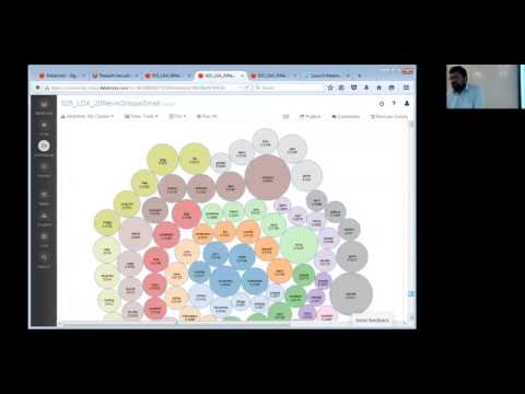
Visualize Results
We will try visualizing the results obtained from the EM LDA model with a d3 bubble chart.
// Zip topic terms with topic IDs
val termArray = topics.zipWithIndex
// Transform data into the form (term, probability, topicId)
val termRDD = sc.parallelize(termArray)
val termRDD2 =termRDD.flatMap( (x: (Array[(String, Double)], Int)) => {
  val arrayOfTuple = x._1
  val topicId = x._2
  arrayOfTuple.map(el => (el._1, el._2, topicId))
})
// Create DF with proper column names
val termDF = termRDD2.toDF.withColumnRenamed("_1", "term").withColumnRenamed("_2", "probability").withColumnRenamed("_3", "topicId")
display(termDF)
We will convert the DataFrame into a JSON format, which will be passed into d3.
// Create JSON data
val rawJson = termDF.toJSON.collect().mkString(",\n")
We are now ready to use D3 on the rawJson data.
displayHTML(s"""
<!DOCTYPE html>
<meta charset="utf-8">
<style>

circle {
  fill: rgb(31, 119, 180);
  fill-opacity: 0.5;
  stroke: rgb(31, 119, 180);
  stroke-width: 1px;
}

.leaf circle {
  fill: #ff7f0e;
  fill-opacity: 1;
}

text {
  font: 14px sans-serif;
}

</style>
<body>
<script src="https://cdnjs.cloudflare.com/ajax/libs/d3/3.5.5/d3.min.js"></script>
<script>

var json = {
 "name": "data",
 "children": [
  {
     "name": "topics",
     "children": [
      ${rawJson}
     ]
    }
   ]
};

var r = 1500,
    format = d3.format(",d"),
    fill = d3.scale.category20c();

var bubble = d3.layout.pack()
    .sort(null)
    .size([r, r])
    .padding(1.5);

var vis = d3.select("body").append("svg")
    .attr("width", r)
    .attr("height", r)
    .attr("class", "bubble");


var node = vis.selectAll("g.node")
    .data(bubble.nodes(classes(json))
    .filter(function(d) { return !d.children; }))
    .enter().append("g")
    .attr("class", "node")
    .attr("transform", function(d) { return "translate(" + d.x + "," + d.y + ")"; })
    color = d3.scale.category20();

  node.append("title")
      .text(function(d) { return d.className + ": " + format(d.value); });

  node.append("circle")
      .attr("r", function(d) { return d.r; })
      .style("fill", function(d) {return color(d.topicName);});

var text = node.append("text")
    .attr("text-anchor", "middle")
    .attr("dy", ".3em")
    .text(function(d) { return d.className.substring(0, d.r / 3)});

  text.append("tspan")
      .attr("dy", "1.2em")
      .attr("x", 0)
      .text(function(d) {return Math.ceil(d.value * 10000) /10000; });

// Returns a flattened hierarchy containing all leaf nodes under the root.
function classes(root) {
  var classes = [];

  function recurse(term, node) {
    if (node.children) node.children.forEach(function(child) { recurse(node.term, child); });
    else classes.push({topicName: node.topicId, className: node.term, value: node.probability});
  }

  recurse(null, root);
  return {children: classes};
}
</script>
""")
You try!
NOW or Later as HOMEWORK Try to do the same process for the State of the Union Addresses dataset from Week1.
As a first step, first locate where that data is… Go to week1 and try to see if each SoU can be treated as a document for topic modeling and whether there is temporal clustering of SoU’s within the same topic.
Try to improve the models (if you want to do a project based on this, perhaps).
Old Bailey, London’s Central Criminal Court, 1674 to 1913
- with Full XML Data for another great project.
displayHTML(frameIt("https://www.oldbaileyonline.org/", 450))
This exciting dataset is here for a fun project:
-
Try the xml-parsing of the dataset already started in Workspace/scalable-data-science/xtraResources -> OldBaileyOnline -> OBO_LoadExtract
-
http://www.math.canterbury.ac.nz/~r.sainudiin/datasets/public/OldBailey/
-
First see Jasper Mackenzie, Raazesh Sainudiin, James Smithies and Heather Wolffram, A nonparametric view of the civilizing process in London’s Old Bailey, Research Report UCDMS2015/1, 32 pages, 2015 (the second revision is in prgress June 2016).
Step 1. Downloading and Loading Data into DBFS
Here are the steps taken for downloading and saving data to the distributed file system. Uncomment them for repeating this process on your databricks cluster or for downloading a new source of data.
//%sh wget http://kdd.ics.uci.edu/databases/20newsgroups/mini_newsgroups.tar.gz -O /tmp/newsgroups.tar.gz
Untar the file into the /tmp/ folder.
//%sh tar xvfz /tmp/newsgroups.tar.gz -C /tmp/
The below cell takes about 10mins to run.
NOTE: It is slow partly because each file is small and we are facing the ‘small files problem’ with distributed file systems that need meta-data for each file. If the file name is not needed then it may be better to create one large stream of the contents of all the files into dbfs. We leave this as it is to show what happens when we upload a dataset of lots of little files into dbfs.
//%fs cp -r file:/tmp/mini_newsgroups dbfs:/datasets/mini_newsgroups
display(dbutils.fs.ls("dbfs:/datasets/mini_newsgroups"))
Scalable Data Science
prepared by Raazesh Sainudiin and Sivanand Sivaram
supported by
and