ScaDaMaLe Course site and book

This is a 2019-2021 augmentation and update of Adam Breindel's initial notebooks.

Thanks to Christian von Koch and William Anzén for their contributions towards making these materials Spark 3.0.1 and Python 3+ compliant.

Convolutional Neural Networks

aka CNN, ConvNet

As a baseline, let's start a lab running with what we already know.

We'll take our deep feed-forward multilayer perceptron network, with ReLU activations and reasonable initializations, and apply it to learning the MNIST digits.

The main part of the code looks like the following (full code you can run is in the next cell):

# imports, setup, load data sets

model = Sequential()
model.add(Dense(20, input_dim=784, kernel_initializer='normal', activation='relu'))
model.add(Dense(15, kernel_initializer='normal', activation='relu'))
model.add(Dense(10, kernel_initializer='normal', activation='softmax'))
model.compile(loss='categorical_crossentropy', optimizer='adam', metrics=['categorical_accuracy'])

categorical_labels = to_categorical(y_train, num_classes=10)

history = model.fit(X_train, categorical_labels, epochs=100, batch_size=100)

# print metrics, plot errors

Note the changes, which are largely about building a classifier instead of a regression model: * Output layer has one neuron per category, with softmax activation * Loss function is cross-entropy loss * Accuracy metric is categorical accuracy

Let's hold pointers into wikipedia for these new concepts.

The following is from: https://www.quora.com/How-does-Keras-calculate-accuracy.

Categorical accuracy:

def categorical_accuracy(y_true, y_pred):
 return K.cast(K.equal(K.argmax(y_true, axis=-1),
 K.argmax(y_pred, axis=-1)),
 K.floatx())

K.argmax(y_true) takes the highest value to be the prediction and matches against the comparative set.

Watch (1:39) *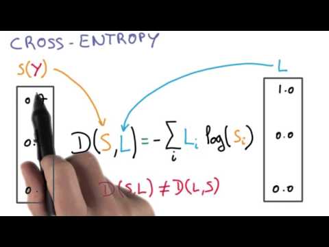

Watch (1:54) *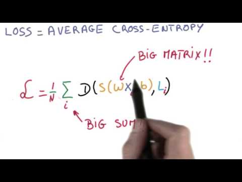

from keras.models import Sequential
from keras.layers import Dense
from keras.utils import to_categorical
import sklearn.datasets
import datetime
import matplotlib.pyplot as plt
import numpy as np

train_libsvm = "/dbfs/databricks-datasets/mnist-digits/data-001/mnist-digits-train.txt"
test_libsvm = "/dbfs/databricks-datasets/mnist-digits/data-001/mnist-digits-test.txt"

X_train, y_train = sklearn.datasets.load_svmlight_file(train_libsvm, n_features=784)
X_train = X_train.toarray()

X_test, y_test = sklearn.datasets.load_svmlight_file(test_libsvm, n_features=784)
X_test = X_test.toarray()

model = Sequential()
model.add(Dense(20, input_dim=784, kernel_initializer='normal', activation='relu'))
model.add(Dense(15, kernel_initializer='normal', activation='relu'))
model.add(Dense(10, kernel_initializer='normal', activation='softmax'))
model.compile(loss='categorical_crossentropy', optimizer='adam', metrics=['categorical_accuracy'])

categorical_labels = to_categorical(y_train, num_classes=10)
start = datetime.datetime.today()

history = model.fit(X_train, categorical_labels, epochs=40, batch_size=100, validation_split=0.1, verbose=2)

scores = model.evaluate(X_test, to_categorical(y_test, num_classes=10))

print
for i in range(len(model.metrics_names)):
	print("%s: %f" % (model.metrics_names[i], scores[i]))

print ("Start: " + str(start))
end = datetime.datetime.today()
print ("End: " + str(end))
print ("Elapse: " + str(end-start))

Using TensorFlow backend.
WARNING:tensorflow:From /databricks/python/lib/python3.7/site-packages/tensorflow/python/framework/op_def_library.py:263: colocate_with (from tensorflow.python.framework.ops) is deprecated and will be removed in a future version.
Instructions for updating:
Colocations handled automatically by placer.
WARNING:tensorflow:From /databricks/python/lib/python3.7/site-packages/tensorflow/python/ops/math_ops.py:3066: to_int32 (from tensorflow.python.ops.math_ops) is deprecated and will be removed in a future version.
Instructions for updating:
Use tf.cast instead.
Train on 54000 samples, validate on 6000 samples
Epoch 1/40
 - 2s - loss: 0.5150 - categorical_accuracy: 0.8445 - val_loss: 0.2426 - val_categorical_accuracy: 0.9282
Epoch 2/40
 - 2s - loss: 0.2352 - categorical_accuracy: 0.9317 - val_loss: 0.1763 - val_categorical_accuracy: 0.9487
Epoch 3/40
 - 2s - loss: 0.1860 - categorical_accuracy: 0.9454 - val_loss: 0.1526 - val_categorical_accuracy: 0.9605
Epoch 4/40
 - 1s - loss: 0.1602 - categorical_accuracy: 0.9527 - val_loss: 0.1600 - val_categorical_accuracy: 0.9573
Epoch 5/40
 - 2s - loss: 0.1421 - categorical_accuracy: 0.9575 - val_loss: 0.1464 - val_categorical_accuracy: 0.9590
Epoch 6/40
 - 1s - loss: 0.1277 - categorical_accuracy: 0.9611 - val_loss: 0.1626 - val_categorical_accuracy: 0.9568
Epoch 7/40
 - 1s - loss: 0.1216 - categorical_accuracy: 0.9610 - val_loss: 0.1263 - val_categorical_accuracy: 0.9665
Epoch 8/40
 - 2s - loss: 0.1136 - categorical_accuracy: 0.9656 - val_loss: 0.1392 - val_categorical_accuracy: 0.9627
Epoch 9/40
 - 2s - loss: 0.1110 - categorical_accuracy: 0.9659 - val_loss: 0.1306 - val_categorical_accuracy: 0.9632
Epoch 10/40
 - 1s - loss: 0.1056 - categorical_accuracy: 0.9678 - val_loss: 0.1298 - val_categorical_accuracy: 0.9643
Epoch 11/40
 - 1s - loss: 0.1010 - categorical_accuracy: 0.9685 - val_loss: 0.1523 - val_categorical_accuracy: 0.9583
Epoch 12/40
 - 2s - loss: 0.1003 - categorical_accuracy: 0.9692 - val_loss: 0.1540 - val_categorical_accuracy: 0.9583
Epoch 13/40
 - 1s - loss: 0.0929 - categorical_accuracy: 0.9713 - val_loss: 0.1348 - val_categorical_accuracy: 0.9647
Epoch 14/40
 - 1s - loss: 0.0898 - categorical_accuracy: 0.9716 - val_loss: 0.1476 - val_categorical_accuracy: 0.9628
Epoch 15/40
 - 1s - loss: 0.0885 - categorical_accuracy: 0.9722 - val_loss: 0.1465 - val_categorical_accuracy: 0.9633
Epoch 16/40
 - 2s - loss: 0.0840 - categorical_accuracy: 0.9736 - val_loss: 0.1584 - val_categorical_accuracy: 0.9623
Epoch 17/40
 - 2s - loss: 0.0844 - categorical_accuracy: 0.9730 - val_loss: 0.1530 - val_categorical_accuracy: 0.9598
Epoch 18/40
 - 2s - loss: 0.0828 - categorical_accuracy: 0.9739 - val_loss: 0.1395 - val_categorical_accuracy: 0.9662
Epoch 19/40
 - 2s - loss: 0.0782 - categorical_accuracy: 0.9755 - val_loss: 0.1640 - val_categorical_accuracy: 0.9623
Epoch 20/40
 - 1s - loss: 0.0770 - categorical_accuracy: 0.9760 - val_loss: 0.1638 - val_categorical_accuracy: 0.9568
Epoch 21/40
 - 1s - loss: 0.0754 - categorical_accuracy: 0.9763 - val_loss: 0.1773 - val_categorical_accuracy: 0.9608
Epoch 22/40
 - 2s - loss: 0.0742 - categorical_accuracy: 0.9769 - val_loss: 0.1767 - val_categorical_accuracy: 0.9603
Epoch 23/40
 - 2s - loss: 0.0762 - categorical_accuracy: 0.9762 - val_loss: 0.1623 - val_categorical_accuracy: 0.9597
Epoch 24/40
 - 1s - loss: 0.0724 - categorical_accuracy: 0.9772 - val_loss: 0.1647 - val_categorical_accuracy: 0.9635
Epoch 25/40
 - 1s - loss: 0.0701 - categorical_accuracy: 0.9781 - val_loss: 0.1705 - val_categorical_accuracy: 0.9623
Epoch 26/40
 - 2s - loss: 0.0702 - categorical_accuracy: 0.9777 - val_loss: 0.1673 - val_categorical_accuracy: 0.9658
Epoch 27/40
 - 2s - loss: 0.0682 - categorical_accuracy: 0.9788 - val_loss: 0.1841 - val_categorical_accuracy: 0.9607
Epoch 28/40
 - 2s - loss: 0.0684 - categorical_accuracy: 0.9790 - val_loss: 0.1738 - val_categorical_accuracy: 0.9623
Epoch 29/40
 - 2s - loss: 0.0670 - categorical_accuracy: 0.9786 - val_loss: 0.1880 - val_categorical_accuracy: 0.9610
Epoch 30/40
 - 2s - loss: 0.0650 - categorical_accuracy: 0.9790 - val_loss: 0.1765 - val_categorical_accuracy: 0.9650
Epoch 31/40
 - 2s - loss: 0.0639 - categorical_accuracy: 0.9793 - val_loss: 0.1774 - val_categorical_accuracy: 0.9602
Epoch 32/40
 - 2s - loss: 0.0660 - categorical_accuracy: 0.9791 - val_loss: 0.1885 - val_categorical_accuracy: 0.9622
Epoch 33/40
 - 1s - loss: 0.0636 - categorical_accuracy: 0.9795 - val_loss: 0.1928 - val_categorical_accuracy: 0.9595
Epoch 34/40
 - 1s - loss: 0.0597 - categorical_accuracy: 0.9805 - val_loss: 0.1948 - val_categorical_accuracy: 0.9593
Epoch 35/40
 - 2s - loss: 0.0631 - categorical_accuracy: 0.9797 - val_loss: 0.2019 - val_categorical_accuracy: 0.9563
Epoch 36/40
 - 2s - loss: 0.0600 - categorical_accuracy: 0.9812 - val_loss: 0.1852 - val_categorical_accuracy: 0.9595
Epoch 37/40
 - 2s - loss: 0.0597 - categorical_accuracy: 0.9812 - val_loss: 0.1794 - val_categorical_accuracy: 0.9637
Epoch 38/40
 - 2s - loss: 0.0588 - categorical_accuracy: 0.9812 - val_loss: 0.1933 - val_categorical_accuracy: 0.9625
Epoch 39/40
 - 2s - loss: 0.0629 - categorical_accuracy: 0.9805 - val_loss: 0.2177 - val_categorical_accuracy: 0.9582
Epoch 40/40
 - 2s - loss: 0.0559 - categorical_accuracy: 0.9828 - val_loss: 0.1875 - val_categorical_accuracy: 0.9642

   32/10000 [..............................] - ETA: 0s
 1568/10000 [===>..........................] - ETA: 0s
 3072/10000 [========>.....................] - ETA: 0s
 4672/10000 [=============>................] - ETA: 0s
 6496/10000 [==================>...........] - ETA: 0s
 8192/10000 [=======================>......] - ETA: 0s
10000/10000 [==============================] - 0s 30us/step
loss: 0.227984
categorical_accuracy: 0.954900
Start: 2021-02-10 10:20:06.310772
End: 2021-02-10 10:21:10.141213
Elapse: 0:01:03.830441

after about a minute we have:

...

Epoch 40/40
1s - loss: 0.0610 - categorical_accuracy: 0.9809 - val_loss: 0.1918 - val_categorical_accuracy: 0.9583

...
 
loss: 0.216120

categorical_accuracy: 0.955000

Start: 2017-12-06 07:35:33.948102

End: 2017-12-06 07:36:27.046130

Elapse: 0:00:53.098028

import matplotlib.pyplot as plt

fig, ax = plt.subplots()
fig.set_size_inches((5,5))
plt.plot(history.history['loss'])
plt.plot(history.history['val_loss'])
plt.title('model loss')
plt.ylabel('loss')
plt.xlabel('epoch')
plt.legend(['train', 'val'], loc='upper left')
display(fig)

What are the big takeaways from this experiment?

We get pretty impressive "apparent error" accuracy right from the start! A small network gets us to training accuracy 97% by epoch 20
The model appears to continue to learn if we let it run, although it does slow down and oscillate a bit.
Our test accuracy is about 95% after 5 epochs and never gets better ... it gets worse!
Therefore, we are overfitting very quickly... most of the "training" turns out to be a waste.
For what it's worth, we get 95% accuracy without much work.

This is not terrible compared to other, non-neural-network approaches to the problem. After all, we could probably tweak this a bit and do even better.

But we talked about using deep learning to solve "95%" problems or "98%" problems ... where one error in 20, or 50 simply won't work. If we can get to "multiple nines" of accuracy, then we can do things like automate mail sorting and translation, create cars that react properly (all the time) to street signs, and control systems for robots or drones that function autonomously.

Try two more experiments (try them separately): 1. Add a third, hidden layer. 2. Increase the size of the hidden layers.

Adding another layer slows things down a little (why?) but doesn't seem to make a difference in accuracy.

Adding a lot more neurons into the first topology slows things down significantly -- 10x as many neurons, and only a marginal increase in accuracy. Notice also (in the plot) that the learning clearly degrades after epoch 50 or so.

... We need a new approach!

... let's think about this:

What is layer 2 learning from layer 1? Combinations of pixels

Combinations of pixels contain information but...

There are a lot of them (combinations) and they are "fragile"

In fact, in our last experiment, we basically built a model that memorizes a bunch of "magic" pixel combinations.

What might be a better way to build features?

When humans perform this task, we look not at arbitrary pixel combinations, but certain geometric patterns -- lines, curves, loops.
These features are made up of combinations of pixels, but they are far from arbitrary
We identify these features regardless of translation, rotation, etc.

Is there a way to get the network to do the same thing?

I.e., in layer one, identify pixels. Then in layer 2+, identify abstractions over pixels that are translation-invariant 2-D shapes?

We could look at where a "filter" that represents one of these features (e.g., and edge) matches the image.

How would this work?

Convolution

Convolution in the general mathematical sense is define as follows:

The convolution we deal with in deep learning is a simplified case. We want to compare two signals. Here are two visualizations, courtesy of Wikipedia, that help communicate how convolution emphasizes features:

Here's an animation (where we change \({\tau}\))

In one sense, the convolution captures and quantifies the pattern matching over space

If we perform this in two dimensions, we can achieve effects like highlighting edges:

The matrix here, also called a convolution kernel, is one of the functions we are convolving. Other convolution kernels can blur, "sharpen," etc.

So we'll drop in a number of convolution kernels, and the network will learn where to use them? Nope. Better than that.

We'll program in the idea of discrete convolution, and the network will learn what kernels extract meaningful features!

The values in a (fixed-size) convolution kernel matrix will be variables in our deep learning model. Although inuitively it seems like it would be hard to learn useful params, in fact, since those variables are used repeatedly across the image data, it "focuses" the error on a smallish number of parameters with a lot of influence -- so it should be vastly less expensive to train than just a huge fully connected layer like we discussed above.

This idea was developed in the late 1980s, and by 1989, Yann LeCun (at AT&T/Bell Labs) had built a practical high-accuracy system (used in the 1990s for processing handwritten checks and mail).

How do we hook this into our neural networks?

First, we can preserve the geometric properties of our data by "shaping" the vectors as 2D instead of 1D.
Then we'll create a layer whose value is not just activation applied to weighted sum of inputs, but instead it's the result of a dot-product (element-wise multiply and sum) between the kernel and a patch of the input vector (image).
- This value will be our "pre-activation" and optionally feed into an activation function (or "detector")

If we perform this operation at lots of positions over the image, we'll get lots of outputs, as many as one for every input pixel.

So we'll add another layer that "picks" the highest convolution pattern match from nearby pixels, which
- makes our pattern match a little bit translation invariant (a fuzzy location match)
- reduces the number of outputs significantly
This layer is commonly called a pooling layer, and if we pick the "maximum match" then it's a "max pooling" layer.

The end result is that the kernel or filter together with max pooling creates a value in a subsequent layer which represents the appearance of a pattern in a local area in a prior layer.

Again, the network will be given a number of "slots" for these filters and will learn (by minimizing error) what filter values produce meaningful features. This is the key insight into how modern image-recognition networks are able to generalize -- i.e., learn to tell 6s from 7s or cats from dogs.

Ok, let's build our first ConvNet:

First, we want to explicity shape our data into a 2-D configuration. We'll end up with a 4-D tensor where the first dimension is the training examples, then each example is 28x28 pixels, and we'll explicitly say it's 1-layer deep. (Why? with color images, we typically process over 3 or 4 channels in this last dimension)

A step by step animation follows: * http://cs231n.github.io/assets/conv-demo/index.html

train_libsvm = "/dbfs/databricks-datasets/mnist-digits/data-001/mnist-digits-train.txt"
test_libsvm = "/dbfs/databricks-datasets/mnist-digits/data-001/mnist-digits-test.txt"

X_train, y_train = sklearn.datasets.load_svmlight_file(train_libsvm, n_features=784)
X_train = X_train.toarray()

X_test, y_test = sklearn.datasets.load_svmlight_file(test_libsvm, n_features=784)
X_test = X_test.toarray()

X_train = X_train.reshape( (X_train.shape[0], 28, 28, 1) )
X_train = X_train.astype('float32')
X_train /= 255
y_train = to_categorical(y_train, num_classes=10)

X_test = X_test.reshape( (X_test.shape[0], 28, 28, 1) )
X_test = X_test.astype('float32')
X_test /= 255
y_test = to_categorical(y_test, num_classes=10)

Now the model:

from keras.layers import Dense, Dropout, Activation, Flatten, Conv2D, MaxPooling2D

model = Sequential()

model.add(Conv2D(8, # number of kernels 
				(4, 4), # kernel size
                padding='valid', # no padding; output will be smaller than input
                input_shape=(28, 28, 1)))

model.add(Activation('relu'))

model.add(MaxPooling2D(pool_size=(2,2)))

model.add(Flatten())
model.add(Dense(128))
model.add(Activation('relu')) # alternative syntax for applying activation

model.add(Dense(10))
model.add(Activation('softmax'))

model.compile(loss='categorical_crossentropy', optimizer='adam', metrics=['accuracy'])

... and the training loop and output:

start = datetime.datetime.today()

history = model.fit(X_train, y_train, batch_size=128, epochs=8, verbose=2, validation_split=0.1)

scores = model.evaluate(X_test, y_test, verbose=1)

print
for i in range(len(model.metrics_names)):
	print("%s: %f" % (model.metrics_names[i], scores[i]))

Train on 54000 samples, validate on 6000 samples
Epoch 1/8
 - 21s - loss: 0.3099 - acc: 0.9143 - val_loss: 0.1025 - val_acc: 0.9728
Epoch 2/8
 - 32s - loss: 0.0972 - acc: 0.9712 - val_loss: 0.0678 - val_acc: 0.9810
Epoch 3/8
 - 35s - loss: 0.0653 - acc: 0.9803 - val_loss: 0.0545 - val_acc: 0.9858
Epoch 4/8
 - 43s - loss: 0.0495 - acc: 0.9852 - val_loss: 0.0503 - val_acc: 0.9865
Epoch 5/8
 - 42s - loss: 0.0392 - acc: 0.9884 - val_loss: 0.0503 - val_acc: 0.9845
Epoch 6/8
 - 41s - loss: 0.0319 - acc: 0.9904 - val_loss: 0.0554 - val_acc: 0.9850
Epoch 7/8
 - 40s - loss: 0.0250 - acc: 0.9927 - val_loss: 0.0437 - val_acc: 0.9885
Epoch 8/8
 - 47s - loss: 0.0226 - acc: 0.9929 - val_loss: 0.0465 - val_acc: 0.9872

   32/10000 [..............................] - ETA: 5s
  160/10000 [..............................] - ETA: 5s
  288/10000 [..............................] - ETA: 4s
  416/10000 [>.............................] - ETA: 4s
  544/10000 [>.............................] - ETA: 4s
  672/10000 [=>............................] - ETA: 4s
  800/10000 [=>............................] - ETA: 4s
  928/10000 [=>............................] - ETA: 4s
 1056/10000 [==>...........................] - ETA: 4s
 1184/10000 [==>...........................] - ETA: 4s
 1280/10000 [==>...........................] - ETA: 4s
 1408/10000 [===>..........................] - ETA: 4s
 1536/10000 [===>..........................] - ETA: 3s
 1664/10000 [===>..........................] - ETA: 3s
 1760/10000 [====>.........................] - ETA: 3s
 1856/10000 [====>.........................] - ETA: 3s
 1984/10000 [====>.........................] - ETA: 3s
 2080/10000 [=====>........................] - ETA: 3s
 2176/10000 [=====>........................] - ETA: 3s
 2272/10000 [=====>........................] - ETA: 3s
 2336/10000 [======>.......................] - ETA: 3s
 2464/10000 [======>.......................] - ETA: 3s
 2528/10000 [======>.......................] - ETA: 3s
 2656/10000 [======>.......................] - ETA: 3s
 2720/10000 [=======>......................] - ETA: 3s
 2848/10000 [=======>......................] - ETA: 3s
 2944/10000 [=======>......................] - ETA: 3s
 3072/10000 [========>.....................] - ETA: 3s
 3200/10000 [========>.....................] - ETA: 3s
 3328/10000 [========>.....................] - ETA: 3s
 3456/10000 [=========>....................] - ETA: 3s
 3584/10000 [=========>....................] - ETA: 3s
 3712/10000 [==========>...................] - ETA: 3s
 3840/10000 [==========>...................] - ETA: 3s
 3968/10000 [==========>...................] - ETA: 3s
 4064/10000 [===========>..................] - ETA: 3s
 4160/10000 [===========>..................] - ETA: 3s
 4256/10000 [===========>..................] - ETA: 3s
 4352/10000 [============>.................] - ETA: 2s
 4416/10000 [============>.................] - ETA: 2s
 4512/10000 [============>.................] - ETA: 2s
 4576/10000 [============>.................] - ETA: 2s
 4704/10000 [=============>................] - ETA: 2s
 4800/10000 [=============>................] - ETA: 2s
 4896/10000 [=============>................] - ETA: 2s
 4928/10000 [=============>................] - ETA: 2s
 5056/10000 [==============>...............] - ETA: 2s
 5152/10000 [==============>...............] - ETA: 2s
 5280/10000 [==============>...............] - ETA: 2s
 5344/10000 [===============>..............] - ETA: 2s
 5472/10000 [===============>..............] - ETA: 2s
 5536/10000 [===============>..............] - ETA: 2s
 5600/10000 [===============>..............] - ETA: 2s
 5728/10000 [================>.............] - ETA: 2s
 5792/10000 [================>.............] - ETA: 2s
 5920/10000 [================>.............] - ETA: 2s
 6016/10000 [=================>............] - ETA: 2s
 6048/10000 [=================>............] - ETA: 2s
 6144/10000 [=================>............] - ETA: 2s
 6240/10000 [=================>............] - ETA: 2s
 6336/10000 [==================>...........] - ETA: 2s
 6464/10000 [==================>...........] - ETA: 2s
 6592/10000 [==================>...........] - ETA: 2s
 6720/10000 [===================>..........] - ETA: 1s
 6816/10000 [===================>..........] - ETA: 1s
 6944/10000 [===================>..........] - ETA: 1s
 7040/10000 [====================>.........] - ETA: 1s
 7168/10000 [====================>.........] - ETA: 1s
 7296/10000 [====================>.........] - ETA: 1s
 7424/10000 [=====================>........] - ETA: 1s
 7552/10000 [=====================>........] - ETA: 1s
 7648/10000 [=====================>........] - ETA: 1s
 7744/10000 [======================>.......] - ETA: 1s
 7840/10000 [======================>.......] - ETA: 1s
 7936/10000 [======================>.......] - ETA: 1s
 8064/10000 [=======================>......] - ETA: 1s
 8128/10000 [=======================>......] - ETA: 1s
 8256/10000 [=======================>......] - ETA: 1s
 8352/10000 [========================>.....] - ETA: 0s
 8480/10000 [========================>.....] - ETA: 0s
 8576/10000 [========================>.....] - ETA: 0s
 8672/10000 [=========================>....] - ETA: 0s
 8768/10000 [=========================>....] - ETA: 0s
 8864/10000 [=========================>....] - ETA: 0s
 8960/10000 [=========================>....] - ETA: 0s
 9056/10000 [==========================>...] - ETA: 0s
 9152/10000 [==========================>...] - ETA: 0s
 9216/10000 [==========================>...] - ETA: 0s
 9344/10000 [===========================>..] - ETA: 0s
 9472/10000 [===========================>..] - ETA: 0s
 9568/10000 [===========================>..] - ETA: 0s
 9632/10000 [===========================>..] - ETA: 0s
 9760/10000 [============================>.] - ETA: 0s
 9856/10000 [============================>.] - ETA: 0s
 9952/10000 [============================>.] - ETA: 0s
10000/10000 [==============================] - 6s 583us/step
loss: 0.040131
acc: 0.986400

fig, ax = plt.subplots()
fig.set_size_inches((5,5))
plt.plot(history.history['loss'])
plt.plot(history.history['val_loss'])
plt.title('model loss')
plt.ylabel('loss')
plt.xlabel('epoch')
plt.legend(['train', 'val'], loc='upper left')
display(fig)

Our MNIST ConvNet

In our first convolutional MNIST experiment, we get to almost 99% validation accuracy in just a few epochs (a minutes or so on CPU)!

The training accuracy is effectively 100%, though, so we've almost completely overfit (i.e., memorized the training data) by this point and need to do a little work if we want to keep learning.

Let's add another convolutional layer:

model = Sequential()

model.add(Conv2D(8, # number of kernels 
						(4, 4), # kernel size
                        padding='valid',
                        input_shape=(28, 28, 1)))

model.add(Activation('relu'))

model.add(Conv2D(8, (4, 4)))
model.add(Activation('relu'))

model.add(MaxPooling2D(pool_size=(2,2)))

model.add(Flatten())
model.add(Dense(128))
model.add(Activation('relu'))

model.add(Dense(10))
model.add(Activation('softmax'))

model.compile(loss='categorical_crossentropy', optimizer='adam', metrics=['accuracy'])

history = model.fit(X_train, y_train, batch_size=128, epochs=15, verbose=2, validation_split=0.1)

scores = model.evaluate(X_test, y_test, verbose=1)

print
for i in range(len(model.metrics_names)):
	print("%s: %f" % (model.metrics_names[i], scores[i]))

Train on 54000 samples, validate on 6000 samples
Epoch 1/15
 - 104s - loss: 0.2681 - acc: 0.9224 - val_loss: 0.0784 - val_acc: 0.9768
Epoch 2/15
 - 116s - loss: 0.0733 - acc: 0.9773 - val_loss: 0.0581 - val_acc: 0.9843
Epoch 3/15
 - 114s - loss: 0.0511 - acc: 0.9847 - val_loss: 0.0435 - val_acc: 0.9873
Epoch 4/15
 - 115s - loss: 0.0391 - acc: 0.9885 - val_loss: 0.0445 - val_acc: 0.9880
Epoch 5/15
 - 105s - loss: 0.0307 - acc: 0.9904 - val_loss: 0.0446 - val_acc: 0.9890
Epoch 6/15
 - 105s - loss: 0.0251 - acc: 0.9923 - val_loss: 0.0465 - val_acc: 0.9875
Epoch 7/15
 - 102s - loss: 0.0193 - acc: 0.9936 - val_loss: 0.0409 - val_acc: 0.9892
Epoch 8/15
 - 100s - loss: 0.0162 - acc: 0.9948 - val_loss: 0.0468 - val_acc: 0.9878
Epoch 9/15
 - 103s - loss: 0.0138 - acc: 0.9956 - val_loss: 0.0447 - val_acc: 0.9893
Epoch 10/15
 - 104s - loss: 0.0122 - acc: 0.9957 - val_loss: 0.0482 - val_acc: 0.9900
Epoch 11/15
 - 102s - loss: 0.0097 - acc: 0.9969 - val_loss: 0.0480 - val_acc: 0.9895
Epoch 12/15
 - 82s - loss: 0.0089 - acc: 0.9970 - val_loss: 0.0532 - val_acc: 0.9882
Epoch 13/15
 - 93s - loss: 0.0080 - acc: 0.9973 - val_loss: 0.0423 - val_acc: 0.9913
Epoch 14/15
 - 92s - loss: 0.0074 - acc: 0.9976 - val_loss: 0.0557 - val_acc: 0.9883
Epoch 15/15
 - 92s - loss: 0.0043 - acc: 0.9987 - val_loss: 0.0529 - val_acc: 0.9902

   32/10000 [..............................] - ETA: 4s
  128/10000 [..............................] - ETA: 6s
  256/10000 [..............................] - ETA: 5s
  352/10000 [>.............................] - ETA: 6s
  448/10000 [>.............................] - ETA: 6s
  512/10000 [>.............................] - ETA: 6s
  608/10000 [>.............................] - ETA: 6s
  736/10000 [=>............................] - ETA: 5s
  800/10000 [=>............................] - ETA: 6s
  896/10000 [=>............................] - ETA: 5s
 1024/10000 [==>...........................] - ETA: 5s
 1120/10000 [==>...........................] - ETA: 5s
 1216/10000 [==>...........................] - ETA: 5s
 1312/10000 [==>...........................] - ETA: 5s
 1408/10000 [===>..........................] - ETA: 5s
 1504/10000 [===>..........................] - ETA: 5s
 1600/10000 [===>..........................] - ETA: 5s
 1664/10000 [===>..........................] - ETA: 5s
 1760/10000 [====>.........................] - ETA: 5s
 1856/10000 [====>.........................] - ETA: 5s
 1952/10000 [====>.........................] - ETA: 5s
 2048/10000 [=====>........................] - ETA: 5s
 2144/10000 [=====>........................] - ETA: 4s
 2240/10000 [=====>........................] - ETA: 4s
 2336/10000 [======>.......................] - ETA: 4s
 2432/10000 [======>.......................] - ETA: 4s
 2496/10000 [======>.......................] - ETA: 4s
 2592/10000 [======>.......................] - ETA: 4s
 2688/10000 [=======>......................] - ETA: 4s
 2784/10000 [=======>......................] - ETA: 4s
 2880/10000 [=======>......................] - ETA: 4s
 2976/10000 [=======>......................] - ETA: 4s
 3072/10000 [========>.....................] - ETA: 4s
 3168/10000 [========>.....................] - ETA: 4s
 3232/10000 [========>.....................] - ETA: 4s
 3360/10000 [=========>....................] - ETA: 4s
 3456/10000 [=========>....................] - ETA: 4s
 3552/10000 [=========>....................] - ETA: 4s
 3648/10000 [=========>....................] - ETA: 3s
 3776/10000 [==========>...................] - ETA: 3s
 3872/10000 [==========>...................] - ETA: 3s
 3968/10000 [==========>...................] - ETA: 3s
 4096/10000 [===========>..................] - ETA: 3s
 4192/10000 [===========>..................] - ETA: 3s
 4288/10000 [===========>..................] - ETA: 3s
 4384/10000 [============>.................] - ETA: 3s
 4480/10000 [============>.................] - ETA: 3s
 4576/10000 [============>.................] - ETA: 3s
 4672/10000 [=============>................] - ETA: 3s
 4768/10000 [=============>................] - ETA: 3s
 4864/10000 [=============>................] - ETA: 3s
 4960/10000 [=============>................] - ETA: 3s
 5024/10000 [==============>...............] - ETA: 3s
 5120/10000 [==============>...............] - ETA: 3s
 5216/10000 [==============>...............] - ETA: 3s
 5312/10000 [==============>...............] - ETA: 2s
 5408/10000 [===============>..............] - ETA: 2s
 5504/10000 [===============>..............] - ETA: 2s
 5600/10000 [===============>..............] - ETA: 2s
 5696/10000 [================>.............] - ETA: 2s
 5792/10000 [================>.............] - ETA: 2s
 5920/10000 [================>.............] - ETA: 2s
 6016/10000 [=================>............] - ETA: 2s
 6080/10000 [=================>............] - ETA: 2s
 6176/10000 [=================>............] - ETA: 2s
 6272/10000 [=================>............] - ETA: 2s
 6368/10000 [==================>...........] - ETA: 2s
 6464/10000 [==================>...........] - ETA: 2s
 6560/10000 [==================>...........] - ETA: 2s
 6656/10000 [==================>...........] - ETA: 2s
 6752/10000 [===================>..........] - ETA: 2s
 6848/10000 [===================>..........] - ETA: 1s
 6912/10000 [===================>..........] - ETA: 1s
 7008/10000 [====================>.........] - ETA: 1s
 7104/10000 [====================>.........] - ETA: 1s
 7200/10000 [====================>.........] - ETA: 1s
 7328/10000 [====================>.........] - ETA: 1s
 7424/10000 [=====================>........] - ETA: 1s
 7552/10000 [=====================>........] - ETA: 1s
 7648/10000 [=====================>........] - ETA: 1s
 7712/10000 [======================>.......] - ETA: 1s
 7776/10000 [======================>.......] - ETA: 1s
 7872/10000 [======================>.......] - ETA: 1s
 7968/10000 [======================>.......] - ETA: 1s
 8032/10000 [=======================>......] - ETA: 1s
 8128/10000 [=======================>......] - ETA: 1s
 8224/10000 [=======================>......] - ETA: 1s
 8288/10000 [=======================>......] - ETA: 1s
 8352/10000 [========================>.....] - ETA: 1s
 8448/10000 [========================>.....] - ETA: 1s
 8544/10000 [========================>.....] - ETA: 0s
 8640/10000 [========================>.....] - ETA: 0s
 8704/10000 [=========================>....] - ETA: 0s
 8800/10000 [=========================>....] - ETA: 0s
 8864/10000 [=========================>....] - ETA: 0s
 8992/10000 [=========================>....] - ETA: 0s
 9056/10000 [==========================>...] - ETA: 0s
 9152/10000 [==========================>...] - ETA: 0s
 9248/10000 [==========================>...] - ETA: 0s
 9344/10000 [===========================>..] - ETA: 0s
 9408/10000 [===========================>..] - ETA: 0s
 9504/10000 [===========================>..] - ETA: 0s
 9600/10000 [===========================>..] - ETA: 0s
 9696/10000 [============================>.] - ETA: 0s
 9792/10000 [============================>.] - ETA: 0s
 9888/10000 [============================>.] - ETA: 0s
 9984/10000 [============================>.] - ETA: 0s
10000/10000 [==============================] - 7s 663us/step
loss: 0.040078
acc: 0.990700

While that's running, let's look at a number of "famous" convolutional networks!

LeNet (Yann LeCun, 1998)

AlexNet (2012)

Back to our labs: Still Overfitting

We're making progress on our test error -- about 99% -- but just a bit for all the additional time, due to the network overfitting the data.

There are a variety of techniques we can take to counter this -- forms of regularization.

Let's try a relatively simple solution solution that works surprisingly well: add a pair of Dropout filters, a layer that randomly omits a fraction of neurons from each training batch (thus exposing each neuron to only part of the training data).

We'll add more convolution kernels but shrink them to 3x3 as well.

model = Sequential()

model.add(Conv2D(32, # number of kernels 
						(3, 3), # kernel size
                        padding='valid',
                        input_shape=(28, 28, 1)))

model.add(Activation('relu'))

model.add(Conv2D(32, (3, 3)))
model.add(Activation('relu'))

model.add(MaxPooling2D(pool_size=(2,2)))

model.add(Dropout(rate=1-0.25)) # <- regularize, new parameter rate added (rate=1-keep_prob)
model.add(Flatten())
model.add(Dense(128))
model.add(Activation('relu'))

model.add(Dropout(rate=1-0.5)) # <-regularize, new parameter rate added (rate=1-keep_prob)
model.add(Dense(10))
model.add(Activation('softmax'))

model.compile(loss='categorical_crossentropy', optimizer='adam', metrics=['accuracy'])
history = model.fit(X_train, y_train, batch_size=128, epochs=15, verbose=2)

scores = model.evaluate(X_test, y_test, verbose=2)

print
for i in range(len(model.metrics_names)):
	print("%s: %f" % (model.metrics_names[i], scores[i]))

WARNING:tensorflow:From /databricks/python/lib/python3.7/site-packages/keras/backend/tensorflow_backend.py:3733: calling dropout (from tensorflow.python.ops.nn_ops) with keep_prob is deprecated and will be removed in a future version.
Instructions for updating:
Please use `rate` instead of `keep_prob`. Rate should be set to `rate = 1 - keep_prob`.
Epoch 1/15
 - 370s - loss: 0.3865 - acc: 0.8783
Epoch 2/15
 - 353s - loss: 0.1604 - acc: 0.9522
Epoch 3/15
 - 334s - loss: 0.1259 - acc: 0.9617
Epoch 4/15
 - 337s - loss: 0.1071 - acc: 0.9666
Epoch 5/15
 - 265s - loss: 0.0982 - acc: 0.9699
Epoch 6/15
 - 250s - loss: 0.0923 - acc: 0.9716
Epoch 7/15
 - 244s - loss: 0.0845 - acc: 0.9740
Epoch 8/15
 - 247s - loss: 0.0811 - acc: 0.9747
Epoch 9/15
 - 246s - loss: 0.0767 - acc: 0.9766
Epoch 10/15
 - 246s - loss: 0.0749 - acc: 0.9764
Epoch 11/15
 - 247s - loss: 0.0708 - acc: 0.9776
Epoch 12/15
 - 244s - loss: 0.0698 - acc: 0.9779
Epoch 13/15
 - 248s - loss: 0.0667 - acc: 0.9794
Epoch 14/15
 - 244s - loss: 0.0653 - acc: 0.9799
Epoch 15/15
 - 249s - loss: 0.0645 - acc: 0.9801
loss: 0.023579
acc: 0.991300

While that's running, let's look at some more recent ConvNet architectures:

ASIDE: Atrous / Dilated Convolutions

An atrous or dilated convolution is a convolution filter with "holes" in it. Effectively, it is a way to enlarge the filter spatially while not adding as many parameters or attending to every element in the input.

Why? Covering a larger input volume allows recognizing coarser-grained patterns; restricting the number of parameters is a way of regularizing or constraining the capacity of the model, making training easier.

Lab Wrapup

From the last lab, you should have a test accuracy of over 99.1%

For one more activity, try changing the optimizer to old-school "sgd" -- just to see how far we've come with these modern gradient descent techniques in the last few years.

Accuracy will end up noticeably worse ... about 96-97% test accuracy. Two key takeaways:

Without a good optimizer, even a very powerful network design may not achieve results
In fact, we could replace the word "optimizer" there with
- initialization
- activation
- regularization
- (etc.)
All of these elements we've been working with operate together in a complex way to determine final performance

Of course this world evolves fast - see the new kid in the CNN block -- capsule networks

Hinton: “The pooling operation used in convolutional neural networks is a big mistake and the fact that it works so well is a disaster.”

Well worth the 8 minute read: * https://medium.com/ai%C2%B3-theory-practice-business/understanding-hintons-capsule-networks-part-i-intuition-b4b559d1159b

To understand deeper: * original paper: https://arxiv.org/abs/1710.09829

Keras capsule network example

More resources

http://www.wildml.com/2015/12/implementing-a-cnn-for-text-classification-in-tensorflow/
https://openai.com/

sds-3.x/ScaDaMaLe