Finding trends in oil price data.
Johannes Graner (LinkedIn), Albert Nilsson (LinkedIn) and Raazesh Sainudiin (LinkedIn)
2020, Uppsala, Sweden
This project was supported by Combient Mix AB through summer internships at:
Combient Competence Centre for Data Engineering Sciences, Department of Mathematics, Uppsala University, Uppsala, Sweden
Resources
This builds on the following library and its antecedents therein to find trends in historical oil prices:
This work was inspired by:
- Antoine Aamennd's texata-2017
- Andrew Morgan's Trend Calculus Library
"./000a_finance_utils"
When dealing with time series, it can be difficult to find a good way to find and analyze trends in the data.
One approach is by using the Trend Calculus algorithm invented by Andrew Morgan. More information about Trend Calculus can be found at https://lamastex.github.io/spark-trend-calculus-examples/.
defined object TrendUtils
import org.lamastex.spark.trendcalculus._
import spark.implicits._
import org.apache.spark.sql._
import org.apache.spark.sql.functions._
import java.sql.Timestamp
import org.lamastex.spark.trendcalculus._
import spark.implicits._
import org.apache.spark.sql._
import org.apache.spark.sql.functions._
import java.sql.Timestamp
The input to the algorithm is data in the format (ticker, time, value). In this example, ticker is "BCOUSD" (Brent Crude Oil), time is given in minutes and value is the closing price for Brent Crude Oil during that minute.
This data is historical data from 2010 to 2019 taken from https://www.histdata.com/ using methods from FX-1-Minute-Data by Philippe Remy. In this notebook, everything is done on static dataframes. We will soon see examples on streaming dataframes.
There are gaps in the data, notably during the weekends when no trading takes place, but this does not affect the algorithm as it is does not place any assumptions on the data other than that time is monotonically increasing.
The window size is set to 2, which is minimal, because we want to retain as much information as possible.
val windowSize = 2
val dataRootPath = TrendUtils.getFx1mPath
val oilDS = spark.read.fx1m(dataRootPath + "bcousd/*.csv.gz").toDF.withColumn("ticker", lit("BCOUSD")).select($"ticker", $"time" as "x", $"close" as "y").as[TickerPoint].orderBy("x")
If we want to look at long term trends, we can use the output time series as input for another iteration. The output contains the points of the input where the trend changes (reversals). This can be repeated several times, resulting in longer term trends.
Here, we look at (up to) 15 iterations of the algorithm. It is no problem if the output of some iteration is too small to find a reversal in the next iteration, since the output will just be an empty dataframe in that case.
val numReversals = 15
val dfWithReversals = new TrendCalculus2(oilDS, windowSize, spark).nReversalsJoinedWithMaxRev(numReversals)
numReversals: Int = 15
dfWithReversals: org.apache.spark.sql.DataFrame = [ticker: string, x: timestamp ... 17 more fields]
dfWithReversals.show(20, false)
+------+-------------------+-----+---------+---------+---------+---------+---------+---------+---------+---------+---------+----------+----------+----------+----------+----------+----------+------+
|ticker|x                  |y    |reversal1|reversal2|reversal3|reversal4|reversal5|reversal6|reversal7|reversal8|reversal9|reversal10|reversal11|reversal12|reversal13|reversal14|reversal15|maxRev|
+------+-------------------+-----+---------+---------+---------+---------+---------+---------+---------+---------+---------+----------+----------+----------+----------+----------+----------+------+
|BCOUSD|2010-11-14 20:15:00|86.74|null     |null     |null     |null     |null     |null     |null     |null     |null     |null      |null      |null      |null      |null      |null      |0     |
|BCOUSD|2010-11-14 20:17:00|86.75|null     |null     |null     |null     |null     |null     |null     |null     |null     |null      |null      |null      |null      |null      |null      |0     |
|BCOUSD|2010-11-14 20:18:00|86.76|-1       |null     |null     |null     |null     |null     |null     |null     |null     |null      |null      |null      |null      |null      |null      |1     |
|BCOUSD|2010-11-14 20:19:00|86.74|null     |null     |null     |null     |null     |null     |null     |null     |null     |null      |null      |null      |null      |null      |null      |0     |
|BCOUSD|2010-11-14 20:21:00|86.74|1        |null     |null     |null     |null     |null     |null     |null     |null     |null      |null      |null      |null      |null      |null      |1     |
|BCOUSD|2010-11-14 20:24:00|86.75|null     |null     |null     |null     |null     |null     |null     |null     |null     |null      |null      |null      |null      |null      |null      |0     |
|BCOUSD|2010-11-14 20:26:00|86.77|null     |null     |null     |null     |null     |null     |null     |null     |null     |null      |null      |null      |null      |null      |null      |0     |
|BCOUSD|2010-11-14 20:27:00|86.75|null     |null     |null     |null     |null     |null     |null     |null     |null     |null      |null      |null      |null      |null      |null      |0     |
|BCOUSD|2010-11-14 20:28:00|86.79|null     |null     |null     |null     |null     |null     |null     |null     |null     |null      |null      |null      |null      |null      |null      |0     |
|BCOUSD|2010-11-14 20:32:00|86.81|null     |null     |null     |null     |null     |null     |null     |null     |null     |null      |null      |null      |null      |null      |null      |0     |
|BCOUSD|2010-11-14 20:33:00|86.81|-1       |null     |null     |null     |null     |null     |null     |null     |null     |null      |null      |null      |null      |null      |null      |1     |
|BCOUSD|2010-11-14 20:34:00|86.81|null     |null     |null     |null     |null     |null     |null     |null     |null     |null      |null      |null      |null      |null      |null      |0     |
|BCOUSD|2010-11-14 20:35:00|86.79|null     |null     |null     |null     |null     |null     |null     |null     |null     |null      |null      |null      |null      |null      |null      |0     |
|BCOUSD|2010-11-14 20:36:00|86.8 |null     |null     |null     |null     |null     |null     |null     |null     |null     |null      |null      |null      |null      |null      |null      |0     |
|BCOUSD|2010-11-14 20:37:00|86.79|null     |null     |null     |null     |null     |null     |null     |null     |null     |null      |null      |null      |null      |null      |null      |0     |
|BCOUSD|2010-11-14 20:38:00|86.79|1        |null     |null     |null     |null     |null     |null     |null     |null     |null      |null      |null      |null      |null      |null      |1     |
|BCOUSD|2010-11-14 20:39:00|86.79|null     |null     |null     |null     |null     |null     |null     |null     |null     |null      |null      |null      |null      |null      |null      |0     |
|BCOUSD|2010-11-14 20:40:00|86.8 |null     |null     |null     |null     |null     |null     |null     |null     |null     |null      |null      |null      |null      |null      |null      |0     |
|BCOUSD|2010-11-14 20:41:00|86.8 |null     |null     |null     |null     |null     |null     |null     |null     |null     |null      |null      |null      |null      |null      |null      |0     |
|BCOUSD|2010-11-14 20:42:00|86.8 |null     |null     |null     |null     |null     |null     |null     |null     |null     |null      |null      |null      |null      |null      |null      |0     |
+------+-------------------+-----+---------+---------+---------+---------+---------+---------+---------+---------+---------+----------+----------+----------+----------+----------+----------+------+
only showing top 20 rows
The number of reversals decrease rapidly as more iterations are done.
dfWithReversals.cache.count
res3: Long = 2859310
(1 to numReversals).foreach( i => println(dfWithReversals.filter(s"reversal$i is not null").count))
775283
253258
93804
37068
15397
6595
2858
1240
530
230
96
45
25
11
6
We write the resulting dataframe to parquet in order to produce visualizations using Python.
val checkPointPath = TrendUtils.getTrendCalculusCheckpointPath
dfWithReversals.write.mode(SaveMode.Overwrite).parquet(checkPointPath + "joinedDSWithMaxRev_new")
dfWithReversals.unpersist
Visualization
The Python library plotly is used to make interactive visualizations.
from plotly.offline import plot
from plotly.graph_objs import *
from datetime import *
checkPointPath = TrendUtils.getTrendCalculusCheckpointPath()
joinedDS = spark.read.parquet(checkPointPath + "joinedDSWithMaxRev_new").orderBy("x")
We check the size of the dataframe to see if it possible to handle locally since plotly is not available for distributed data.
joinedDS.count()
Almost 3 million rows might be too much for the driver! The timeseries has to be thinned out in order to display locally.
No information about higher order trend reversals is lost since every higher order reversal is also a lower order reversal and the lowest orders of reversal are on the scale of minutes (maybe hours) and that is probably not very interesting considering that the data stretches over roughly 10 years!
joinedDS.filter("maxRev > 2").count()
Just shy of 100k rows is no problem for the driver.
We select the relevant information in the dataframe for visualization.
fullTS = joinedDS.filter("maxRev > 2").select("x","y","maxRev").collect()
Picking an interval to focus on.
Start and end dates as (year, month, day, hour, minute, second). Only year, month and day are required. The interval from years 1800 to 2200 ensures all data is selected.
startDate = datetime(1800,1,1)
endDate= datetime(2200,12,31)
TS = [row for row in fullTS if startDate <= row['x'] and row['x'] <= endDate]
Setting up the visualization.
numReversals = 15
startReversal = 7

allData = {'x': [row['x'] for row in TS], 'y': [row['y'] for row in TS], 'maxRev': [row['maxRev'] for row in TS]}
revTS = [row for row in TS if row[2] >= startReversal]
colorList = ['rgba(' + str(tmp) + ',' + str(255-tmp) + ',' + str(255-tmp) + ',1)' for tmp in [int(i*255/(numReversals-startReversal+1)) for i in range(1,numReversals-startReversal+2)]]

def getRevTS(tsWithRevMax, revMax):
  x = [row[0] for row in tsWithRevMax if row[2] >= revMax]
  y = [row[1] for row in tsWithRevMax if row[2] >= revMax]
  return x,y,revMax

reducedData = [getRevTS(revTS, i) for i in range(startReversal, numReversals+1)]

markerPlots = [Scattergl(x=x, y=y, mode='markers', marker=dict(color=colorList[i-startReversal], size=i), name='Reversal ' + str(i)) for (x,y,i) in [getRevTS(revTS, i) for i in range(startReversal, numReversals+1)]]
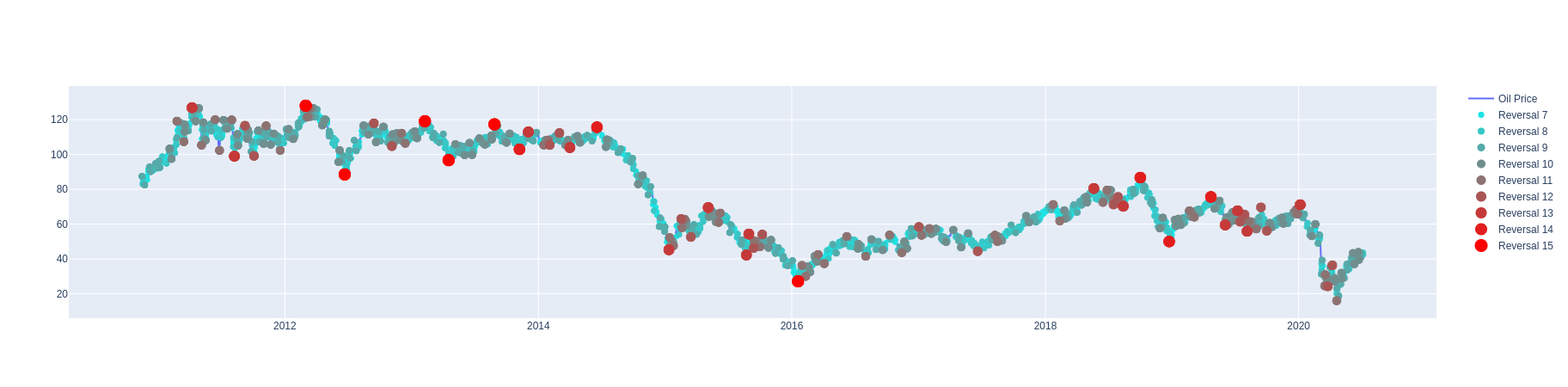
Plotting result as plotly graph
The graph is interactive, one can drag to zoom in on an area (double-click to get back) and click on the legend to hide or show different series.
Note that we have left out many of the lower order reversals in order to not make the graph too cluttered. The seventh order reversal (the lowest order shown) is still on the scale of hours to a few days.
p = plot(
  [Scattergl(x=allData['x'], y=allData['y'], mode='lines', name='Oil Price')] + markerPlots
  ,
  output_type='div'
)

displayHTML(p)