Predicting the load in wireless networks
Project members:
- Sofia Ek, Department of Information Technology, Uppsala University
- Oscar Stenhammar, Network and System Engineering, KTH and Ericsson

Background
Due to the Russian invasion of Ukraine, there is a current global energy crisis all over Europe. Energy prices has gone through the roof causing consumers, as well as industries, to save energy. By saving energy, the energy bill is reduced. For economic reasons industries has been forced to shut down parts of their production line the past months. Another reason for saving energy is to reduce the cost of 1kWh. By lowering the demand, the energy supply will increase. This will force the market to reduce the energy price. To incorporate this, goverments and the EU has put constraints on several industries to surpress the energy consumption. One of these industries are network operators. The constraints might even force them to shut down a few base stations for shorter periods.
With this in mind, how can network operators save energy with minimal impact on end users? This project has been focusing on one solution, to predict the network load. Based on hte predictions of the network load, a decision algorithm could be implemented that could put cells and base stations into sleep mode if the load is expected to be sufficiently low. Sleep functions already exists in 5G networks but are rarely used and could be exploited much further to optimie energy consumptions.
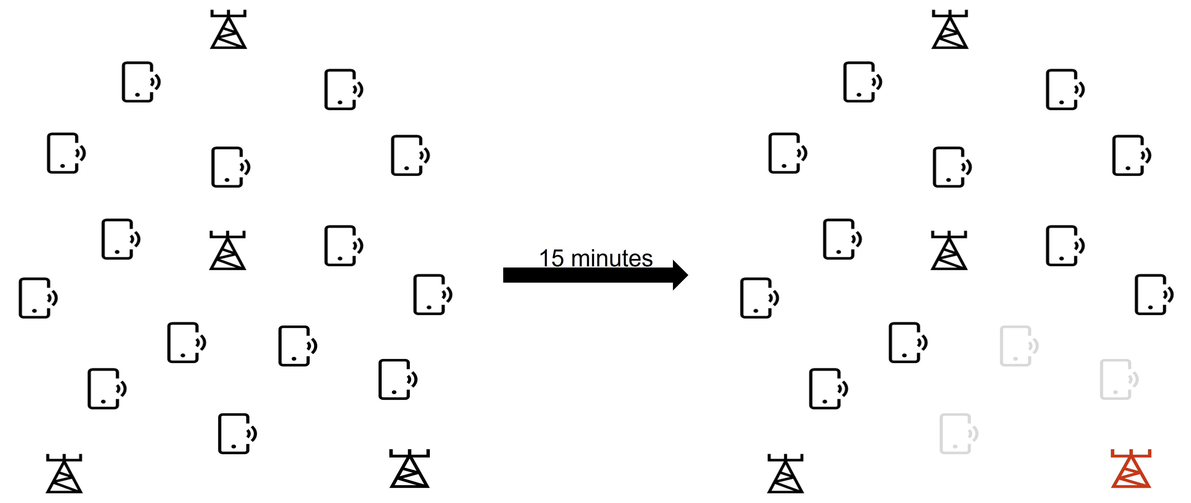
Dataset
- The data is from a network vendor in Europe in an urban environment
- It has been collected in September and October in 2022
- One measurement every 15 minutes, which is a sum of the past 15 minutes.
- There are in total 308 different cells in the dataset
- The dataset contains information about:
- Cell IDs
- Location
- Frequency band
- Throughput volume on the downlink
- Number of active users in each cell.
- The cell ID and the location are anonymized, but the relative location to other cells is still valid.
An example of the first 10 rows of data can be seen below.
# To illustrate the dataset, it is loaded from the next notebook, which fuctionalities will be further explained there.
%run "./01_prepare_data"
df = spark_read_data(True)
Plotting the relative location of the cells:
import matplotlib.pyplot as plt
import seaborn as sns
import pandas as pd
import numpy as np

import warnings
warnings.filterwarnings("ignore")

sns.set(
    context='paper',
    font_scale=1,
    style='ticks',
    rc={
        'lines.linewidth': 2,
        'figure.figsize': (15,12),
        'font.size': 60,
        'lines.markersize': 8,
        'axes.labelsize': 20,
        'xtick.labelsize': 16,
        'ytick.labelsize': 16,
        'legend.fontsize': 16,
        'axes.labelpad': 6
    }
)

df_p = df.where(df.rdiTimeStamp == '2022-09-02 00:00:00').toPandas()
df_p.longitude = df_p.longitude - (df_p.longitude.min() + df_p.longitude.max())/2
df_p.latitude = 111*df_p.latitude + np.random.random(len(df_p))/20
df_p.longitude = 111*df_p.longitude + np.random.random(len(df_p))/20

fig, ax = plt.subplots()
sns.scatterplot(data=df_p, x='longitude', y='latitude', hue='locationIndex')
ax.set_xlabel('X-position [km]')
ax.set_ylabel('Y-position [km]')

plt.legend('',frameon=False)
plt.tight_layout()
plt.show()
For one of the cells in the dataset: A plot of the downlink volume (MB) and the number of users during 24 hours.
df_c = df.where(df.cellId == 1).toPandas()

df_d = df_c[df_c['rdiTimeStamp']<'2022-09-02']
df_d = df_d[df_d['rdiTimeStamp']>'2022-08-30']
df_d = df_d.sort_values(['rdiTimeStamp'])
df_d['pmRadioThpVolDl'] = df_d['pmRadioThpVolDl']/8000
df_d['rdiTimeStamp'] = pd.to_datetime(df_d.rdiTimeStamp)

fig, ax = plt.subplots()
sns.lineplot(ax = ax, data=df_d, x='rdiTimeStamp', y='pmRadioThpVolDl', label='Volume')

ax.set_xlabel('Time [mm-dd HH]')
ax.set_ylabel('Downlink volume [MB]')
ax.set_xticklabels(ax.get_xticklabels(), rotation=25)
ax.legend(loc="upper left")

ax1 = ax.twinx()
ax1.plot(df_d['rdiTimeStamp'], df_d['pmActiveUeDlSum'], color='black', label='Users')
ax1.legend(loc="upper right")
ax1.set_ylabel('Number of users')

plt.tight_layout()
plt.show()
Methods
We focus on three methods: 1. Autoregressiv model (AR-model) 2. Long short-term memory (LSTM) 3. Gated Recurrent Unit (GRU)
We try to predict the throughput volume on the downlink, i.e. the variable called pmRadioThpVolDl.
AR-model: This model is used as a baseline and the model is estimated with linear regression. In this case, we filter the data and only focus on one cell at the time. The model is:
\(y(t) = \beta_1 y(t - 1) + \beta_2 y(t - 2) + \beta_3 y(t - 3) + \beta_4 y(t - 96)\), where y is pmRadioThpVolDl.
LSTM and GRU: These recurrent neural network models uses all the data and creates a global model for prediction. The models are built with Keras/Tensorflow and the training is distributed using Horovod.
More details on our setup will come in the following notebooks.
References:
How to setup linear regression with pyspark: https://towardsdatascience.com/building-a-linear-regression-with-pyspark-and-mllib-d065c3ba246a
Tutoial Horovod and Tensorflow: https://learn.microsoft.com/en-us/azure/synapse-analytics/machine-learning/tutorial-horovod-tensorflow