Distributed Reinforcement Learning
Project members:
- Johan Edstedt, Linköping University
- Arvi Jonnarth, Linköping University & Husqvarna Group
- Yushan Zhang, Linköping University
Presentation:
Project description
We extend the Proximal Policy Optimization (PPO) and Soft Actor-Critic (SAC) reinforcement learning algorithms from the stable_baselines3 library to make them run in a distributed fashion.
We use Horovod, which is a distributed deep learning training framework that supports several ML libraries, including PyTorch through the horovod.torch package. But more importantly, it can be run on top of spark using sparkdl.HorovodRunner. The HorovodRunner launches spark jobs on training functions that implement the Horovod framework. All that is needed to utilize the Horovod framework is to wrap the original torch.optim.Optimizer optimizer in a horovod.torch.DistributedOptimizer.
Reinforcement Learning
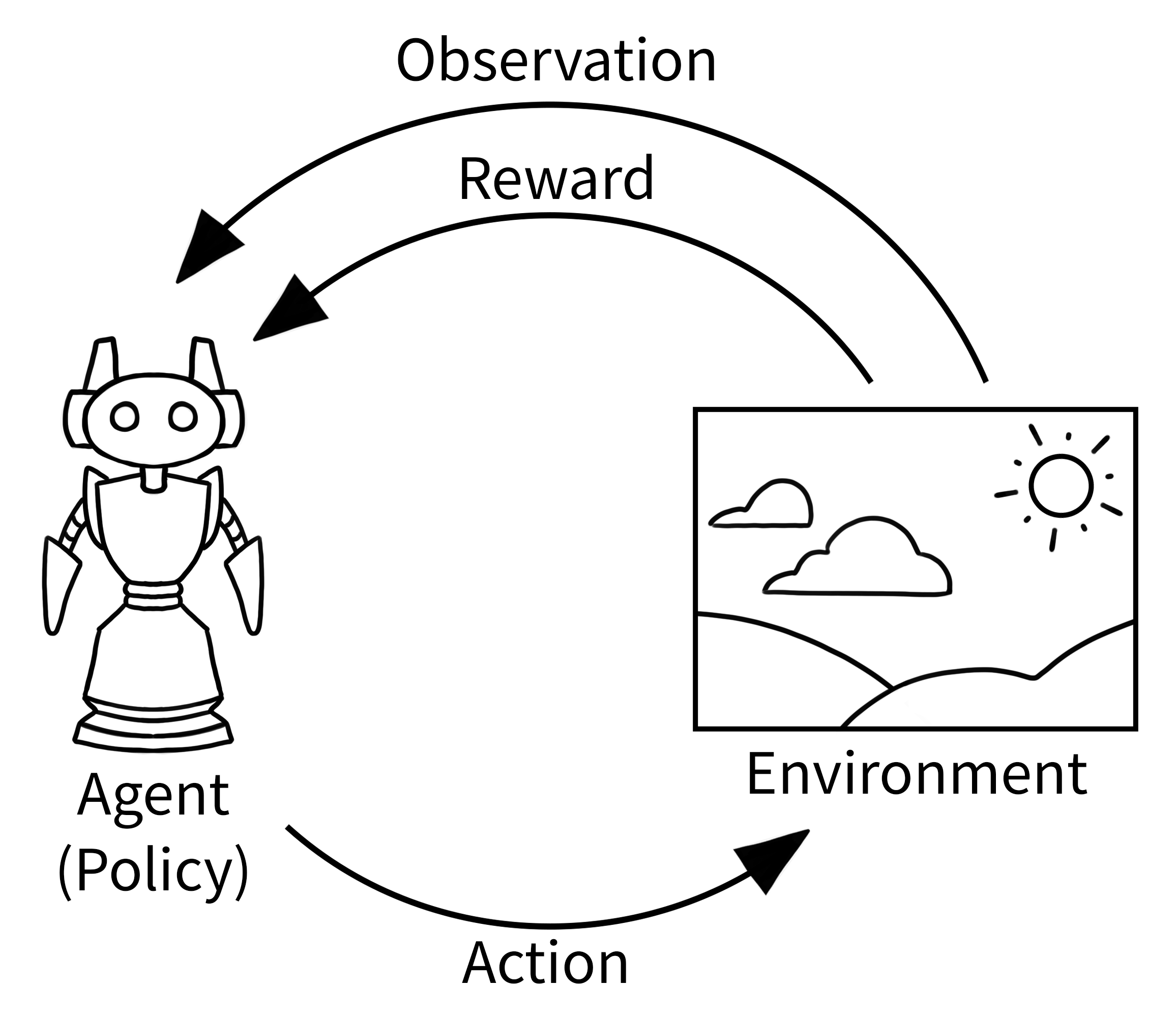
Definition: Reinforcement Learning is one of three basic machine learning paradigms, alongside supervised learning and unsupervised learning. It is a machine learning training method based on rewarding desired behaviors and/or punishing undesired ones. In general, a reinforcement learning agent is able to perceive and interpret its environment, take actions and learn through trial and error.
Environment: Gymnasium, where the classic “agent-environment loop” is implemented. The agent performs some actions in the environment (usually by passing some control inputs to the environment, e.g. torque inputs of motors) and observes how the environment’s state changes. One such action-observation exchange is referred to as a timestep.
Example tasks:


Stable Baselines3
Stable Baselines3 is a set of reliable implementations of reinforcement learning algorithms in PyTorch. It is the latest major version of Stable Baselines.
Github repository: https://github.com/DLR-RM/stable-baselines3
Paper: https://jmlr.org/papers/volume22/20-1364/20-1364.pdf
PPO:
The Proximal Policy Optimization algorithm combines ideas from A2C (having multiple workers) and TRPO (it uses a trust region to improve the actor).
The main idea is that after an update, the new policy should be not too far from the old policy. For that, ppo uses clipping to avoid too large update.
SAC:
Soft Actor Critic (SAC) Off-Policy Maximum Entropy Deep Reinforcement Learning with a Stochastic Actor.
SAC is the successor of Soft Q-Learning SQL and incorporates the double Q-learning trick from TD3. A key feature of SAC, and a major difference with common RL algorithms, is that it is trained to maximize a trade-off between expected return and entropy, a measure of randomness in the policy.
Get all necessary imports.
import csv
import gym
import horovod.torch as hvd
import numpy as np
import os
import shutil
import torch as th
import warnings

from datetime import datetime
from gym import spaces
from matplotlib import pyplot as plt
from sparkdl import HorovodRunner
from torch.nn import functional as F
from typing import Any, Dict, List, Optional, Tuple, Type, TypeVar, Union

from stable_baselines3 import PPO, SAC
from stable_baselines3.common.buffers import ReplayBuffer
from stable_baselines3.common.monitor import Monitor
from stable_baselines3.common.noise import ActionNoise
from stable_baselines3.common.policies import ActorCriticCnnPolicy, ActorCriticPolicy, BasePolicy, MultiInputActorCriticPolicy
from stable_baselines3.common.type_aliases import GymEnv, MaybeCallback, Schedule
from stable_baselines3.common.utils import explained_variance, get_parameters_by_name, get_schedule_fn, polyak_update
from stable_baselines3.sac.policies import CnnPolicy, MlpPolicy, MultiInputPolicy, SACPolicy
And global variables
LOG_DIR = '/dbfs/drl_logs'
Distributed Proximal Policy Optimization, DPPO
Theoretical Background
PPO is a reinforcement learning algorithm, which is trained using the following objective (that should be maximized)
\[ L^{\text{CLIP}}(\theta) = \mathbb E_t \big[ \text{min}(r_t(\theta)A_t, \text{clip}(r_t(\theta), 1-\epsilon, 1+\epsilon)A_t) \big], \]
let's go through what this means. First, \(\pi_{\theta}(a_t|s_t)\) is the "policy". This is a neural network that we want to train to estimate the "best" action to take in any given state. Then we have \(r_t(\theta) = \frac{\pi_{\theta}(a_t | s_t)}{\pi_{\theta_{\text{old}}}(a_t | s_t)}\), which is the ratio of the probability of the network choosing a certain action, compared to a previous version of the network. Then we have \(A_t = -V(s_t) + r_t + \gamma r_{t+1} ...\) which is the estimated advantage. Intuitively this is how much better the policy performed than expected by the value network V. The inituition is that we want to get as large advantages as possible, and it is especially important when the previous policy was unlikely to have yielded the result. However, we still want the new parameters too not go too far from the old ones. To ensure this we "clip" the ratio. This ensures that the policy network gets no gradients after a certain threshold epsilon. See image below:

Here it is clear that the network will cease getting gradient after improving sufficiently on for all timesteps t. A further detail is that the value network has an additional value loss which is trained to minimize the advantage. The algorithm can be summarized as follows.
- Gather a "dataset" of state action reward pairs, given the current policy. (Hereafter referred to as rollouts)
- Train the policy to maximize advantage while clipping, also train the value network to predict the values for accurate estimation of advantage. (Hereafter training)
Practical Implementation
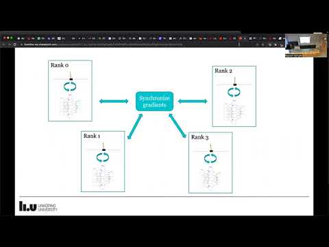
Looking at the above algorithm it is immediately obvious that the rollouts are embarassingly parallel, since no communication is needed between nodes. However, during training, the parameters of the models are updated according to the optimizer (which requires gradients to be synched between nodes). One further caveat: The stable_baselines3 implementation uses inplace gradient clipping. This is a non-linear operation, which means that the sum of clipped gradients over the nodes is not the same as the clipped summed gradient. Hence we first need to sync (sum) the gradients, and then perform clipping. Horovod by default syncs the gradients at optimizer.step(), however it also permits manual syncing, which we have implemented in the code below. We summarize the communication needed between nodes during rollouts and training in the figure below:

We extend the original PPO class from stable_baselines3. We modify the _setup_model function to wrap the optimizer in a hvd.DistributedOptimizer. We also had to change the train function which performs the gradient step. This change was necessary to account for the gradient clipping, which must happen after averaging the gradients across machines.
class DPPO(PPO):
    """
    Distributed Proximal Policy Optimization (DPPO)
    """

    def _setup_model(self) -> None:
        super()._setup_model()
        self.policy.optimizer = hvd.DistributedOptimizer(self.policy.optimizer, named_parameters=self.policy.named_parameters())
        hvd.broadcast_parameters(self.policy.state_dict(), root_rank=0)
        hvd.broadcast_optimizer_state(self.policy.optimizer, root_rank=0)

    def train(self) -> None:
        """
        Update policy using the currently gathered rollout buffer.
        """
        # Switch to train mode (this affects batch norm / dropout)
        self.policy.set_training_mode(True)
        # Update optimizer learning rate
        self._update_learning_rate(self.policy.optimizer)
        # Compute current clip range
        clip_range = self.clip_range(self._current_progress_remaining)
        # Optional: clip range for the value function
        if self.clip_range_vf is not None:
            clip_range_vf = self.clip_range_vf(self._current_progress_remaining)

        entropy_losses = []
        pg_losses, value_losses = [], []
        clip_fractions = []

        continue_training = True

        # train for n_epochs epochs
        for epoch in range(self.n_epochs):
            approx_kl_divs = []
            # Do a complete pass on the rollout buffer
            for rollout_data in self.rollout_buffer.get(self.batch_size):
                actions = rollout_data.actions
                if isinstance(self.action_space, spaces.Discrete):
                    # Convert discrete action from float to long
                    actions = rollout_data.actions.long().flatten()

                # Re-sample the noise matrix because the log_std has changed
                if self.use_sde:
                    self.policy.reset_noise(self.batch_size)

                values, log_prob, entropy = self.policy.evaluate_actions(rollout_data.observations, actions)
                values = values.flatten()
                # Normalize advantage
                advantages = rollout_data.advantages
                # Normalization does not make sense if mini batchsize == 1, see GH issue #325
                if self.normalize_advantage and len(advantages) > 1:
                    advantages = (advantages - advantages.mean()) / (advantages.std() + 1e-8)

                # ratio between old and new policy, should be one at the first iteration
                ratio = th.exp(log_prob - rollout_data.old_log_prob)

                # clipped surrogate loss
                policy_loss_1 = advantages * ratio
                policy_loss_2 = advantages * th.clamp(ratio, 1 - clip_range, 1 + clip_range)
                policy_loss = -th.min(policy_loss_1, policy_loss_2).mean()

                # Logging
                pg_losses.append(policy_loss.item())
                clip_fraction = th.mean((th.abs(ratio - 1) > clip_range).float()).item()
                clip_fractions.append(clip_fraction)

                if self.clip_range_vf is None:
                    # No clipping
                    values_pred = values
                else:
                    # Clip the difference between old and new value
                    # NOTE: this depends on the reward scaling
                    values_pred = rollout_data.old_values + th.clamp(
                        values - rollout_data.old_values, -clip_range_vf, clip_range_vf
                    )
                # Value loss using the TD(gae_lambda) target
                value_loss = F.mse_loss(rollout_data.returns, values_pred)
                value_losses.append(value_loss.item())

                # Entropy loss favor exploration
                if entropy is None:
                    # Approximate entropy when no analytical form
                    entropy_loss = -th.mean(-log_prob)
                else:
                    entropy_loss = -th.mean(entropy)

                entropy_losses.append(entropy_loss.item())

                loss = policy_loss + self.ent_coef * entropy_loss + self.vf_coef * value_loss

                # Calculate approximate form of reverse KL Divergence for early stopping
                # see issue #417: https://github.com/DLR-RM/stable-baselines3/issues/417
                # and discussion in PR #419: https://github.com/DLR-RM/stable-baselines3/pull/419
                # and Schulman blog: http://joschu.net/blog/kl-approx.html
                with th.no_grad():
                    log_ratio = log_prob - rollout_data.old_log_prob
                    approx_kl_div = th.mean((th.exp(log_ratio) - 1) - log_ratio).cpu().numpy()
                    approx_kl_divs.append(approx_kl_div)

                if self.target_kl is not None and approx_kl_div > 1.5 * self.target_kl:
                    continue_training = False
                    if self.verbose >= 1:
                        print(f"Early stopping at step {epoch} due to reaching max kl: {approx_kl_div:.2f}")
                    break

                # Optimization step
                self.policy.optimizer.zero_grad()
                loss.backward()
                # Need to synch gradients first, to prevent non-linear gradient clipping to happen too early
                self.policy.optimizer.synchronize()
                # Clip grad norm
                th.nn.utils.clip_grad_norm_(self.policy.parameters(), self.max_grad_norm)
                # Dont need to sync now.
                with self.policy.optimizer.skip_synchronize():
                    self.policy.optimizer.step()

            if not continue_training:
                break

        self._n_updates += self.n_epochs
        explained_var = explained_variance(self.rollout_buffer.values.flatten(), self.rollout_buffer.returns.flatten())

        # Logs
        self.logger.record("train/entropy_loss", np.mean(entropy_losses))
        self.logger.record("train/policy_gradient_loss", np.mean(pg_losses))
        self.logger.record("train/value_loss", np.mean(value_losses))
        self.logger.record("train/approx_kl", np.mean(approx_kl_divs))
        self.logger.record("train/clip_fraction", np.mean(clip_fractions))
        self.logger.record("train/loss", loss.item())
        self.logger.record("train/explained_variance", explained_var)
        if hasattr(self.policy, "log_std"):
            self.logger.record("train/std", th.exp(self.policy.log_std).mean().item())

        self.logger.record("train/n_updates", self._n_updates, exclude="tensorboard")
        self.logger.record("train/clip_range", clip_range)
        if self.clip_range_vf is not None:
            self.logger.record("train/clip_range_vf", clip_range_vf)
Next, we define our distributed training function that Horovod will run on each process. We make it general since we want to use it for different algorithms. It takes an algorithm class algo as input. Furthermore, it takes the environment name, type of policy, and the number of time steps, as well as any keyword arguments to be passed to the algorithm class. We do any logging or model saving only on the main process, i.e. rank 0.
def train_hvd(algo, env_name="Pendulum-v1", policy="MlpPolicy", total_timesteps=100_000, **kwargs):

    # Initialize Horovod
    hvd.init()

    # Create environment, model, and run training
    env = gym.make(env_name)
    # log reward etc. only on the main process by wrapping the environment in a Monior
    if hvd.rank() == 0:
        env = Monitor(env, os.path.join(LOG_DIR, env_name, algo.__name__ + '-' + str(hvd.size())))
    model = algo(policy, env, **kwargs)
    model.learn(total_timesteps=total_timesteps, log_interval=1)

    # Save model only on process 0
    if hvd.rank() == 0:
        exp_time = datetime.now().strftime('%Y-%m-%d_%H%M%S')
        log_dir = os.path.join(LOG_DIR, exp_time)
        if not os.path.exists(log_dir):
            os.makedirs(log_dir)
        # DBFS doesnt support zip, need to create on driver and then move file to DBFS
        filename = f'{algo.__name__}_{env_name}.zip'
        model.save(filename)
        shutil.move(filename, f"{log_dir}/")

    env.close()
Single-process PPO
First, let us train a PPO agent in a single process using the original implementation from stable_baselines3 (i.e. not using our DPPO class or train_hvd function).
Start with some parameters:
# The environment where to test our distributed PPO algorithm
ppo_env_name = 'CartPole-v1'
#ppo_env_name = 'Pendulum-v1'
#ppo_env_name = 'MountainCarContinuous-v0'
#ppo_env_name = 'BipedalWalker-v3'

# PPO parameters
ppo_total_timesteps = 100_000
ppo_learning_rate = 1e-3 # default: 3e-4
ppo_n_steps = 4096 * 8 # default: 2048
ppo_batch_size = 4096 # default: 64

# How many processes to use for distributed training
ppo_world_sizes = [1, 2, 4, 8]
Train the PPO agent.
# Create a gym environment and wrap it in a Monitor to track the reward
env = gym.make(ppo_env_name)
env = Monitor(env, os.path.join(LOG_DIR, ppo_env_name, 'PPO'))

# Define our PPO agent
model = PPO(
    "MlpPolicy",
    env,
    learning_rate=ppo_learning_rate,
    n_steps=ppo_n_steps,
    batch_size=ppo_batch_size,
    verbose=1)

# Train our agent
model.learn(total_timesteps=ppo_total_timesteps, log_interval=1)
env.close()
Multi-process DPPO
Train our distributed DPPO algorithm for different number of processes (world_size). To have comparable training settings for different number of processes, we divide the per-process rollout buffer size n_steps with the number of processes (since the total buffer size will then be the same). We also multiply the learning rate learning_rate with the number of processes (since the total batch size will be larger). Note that this means that a gradient step for the multi-process case will essentially be equivalent to world_size number of single-process gradient steps. We will take this into account when plotting the results later to validate that the training settings actually are equivalent.
# Loop over number of processes and do an experiment for each
for world_size in ppo_world_sizes:

    # Initialize the HorovodRunner
    hr = HorovodRunner(np=world_size, driver_log_verbosity='all')

    # Launch the spark job on our training function
    hr.run(
        train_hvd,
        algo = DPPO,
        env_name = ppo_env_name,
        policy = "MlpPolicy",
        total_timesteps = ppo_total_timesteps,
        learning_rate = ppo_learning_rate * world_size,
        n_steps = ppo_n_steps // world_size,
        batch_size = ppo_batch_size,
        verbose = 1
    )
PPO and DPPO results
We compare the different runs by plotting the reward over per-process training steps, total number of training steps, and wall time. We expect a faster convergence rate for a larger number of processes when looking at the per-process training steps, and the same reward for the same number of total training steps, since these should correspond to the same training setting. We also expect a faster convergence in wall time for more processes. We also compute the speedup for different number of processes.
Define a function to get the logs from a run.
def get_logs(log_file, as_dict=False):
    steps, rewards, ep_lengths, times = [], [], [], []
    with open(log_file) as csv_file:
        csv_reader = csv.reader(csv_file, delimiter=',')
        for i, row in enumerate(csv_reader):
            if i < 2: # skip first two rows (headers)
                continue
            rewards.append(float(row[0]))
            ep_lengths.append(int(row[1]))
            times.append(float(row[2]))
            steps.append((steps[-1] if len(steps) != 0 else 0) + ep_lengths[-1])
    if as_dict:
        return {'steps': steps,
                'rewards': rewards,
                'ep_lengths': ep_lengths,
                'times': times}
    return steps, rewards, ep_lengths, times
Define a function to plot the reward.
def plot_results(env_name, algo_names, x_axis='steps', num_procs=None, smooth=None):

    # Read logs
    logs = {}
    if isinstance(algo_names, str):
        logs[algo_names] = get_logs(os.path.join(LOG_DIR, env_name, f'{algo_names}.monitor.csv'), as_dict=True)
    else: # list of str
        for algo_name in algo_names:
            logs[algo_name] = get_logs(os.path.join(LOG_DIR, env_name, f'{algo_name}.monitor.csv'), as_dict=True)

    # Plot reward
    for algo_name in algo_names:

        # Scale x-axis if number of processes is given
        if num_procs is not None:
            scale_by_num_proc = num_procs[algo_name]
        else:
            scale_by_num_proc = 1

        # Smooth and plot the reward
        reward = logs[algo_name]['rewards']
        if smooth is not None:
            reward = [reward[0]]*smooth + reward + [reward[-1]]*smooth
            reward = np.convolve(reward, [1/(smooth*2 + 1)]*(smooth*2 + 1), mode='valid')
        plt.plot(scale_by_num_proc*np.array(logs[algo_name][x_axis]), reward)

    plt.legend(algo_names)
    plt.title(env_name)
    plt.ylabel('reward')
    if x_axis == 'times':
        if num_procs is not None:
            plt.xlabel('total cpu time [s]')
        else:
            plt.xlabel('wall time [s]')
    elif x_axis == 'steps':
        if num_procs is not None:
            plt.xlabel('total steps')
        else:
            plt.xlabel('steps per process')
    else:
        plt.xlabel(x_axis)
    plt.gcf().set_size_inches(8, 4)
    plt.show()
Define a function to plot the speedup.
def plot_speedup(env_name, runs):
    algo_name = runs[0]

    # Compute wall time, total steps, and speedup
    wall_times = []
    total_steps = []
    speedups = []
    nprocs = []

    # Get logs from single-process run
    logs1 = get_logs(os.path.join(LOG_DIR, env_name, f'D{algo_name}-1.monitor.csv'), as_dict=True)
    wall_time1 = logs1['times'][-1]
    total_step1 = logs1['steps'][-1]

    # Compute results for each run
    for run in runs:
        logs = get_logs(os.path.join(LOG_DIR, env_name, f'{run}.monitor.csv'), as_dict=True)
        wall_times.append(logs['times'][-1])
        total_steps.append(logs['steps'][-1])
        if '-' in run:
            nprocs.append(int(run.split('-')[1]))
            total_steps[-1] *= nprocs[-1]
            speedup = wall_time1 / wall_times[-1]
            speedup *= total_steps[-1] / total_step1 # adjust for different total steps
            speedups.append(round(speedup, 2))

    # Print run times and total steps
    print('Run times')
    for run, wall_time, total_step in zip(runs, wall_times, total_steps):
        print(f'{run}: {round(wall_time, 2)} s ({total_step} total steps)')

    # Print speedup
    print('\nSpeedups')
    for speedup, nproc in zip(speedups, nprocs):
        print(f'D{algo_name}-{nproc}: {speedup}')

    # Plot speedup as a bar plot
    x = np.arange(len(speedups))  # the label locations
    width = 0.35  # the width of the bars
    fig, ax = plt.subplots()
    rects1 = ax.bar(x - width/2, speedups, width, label='speedup')
    rects2 = ax.bar(x + width/2, nprocs, width, label='ideal')

    # Add some text for labels, title and custom x-axis tick labels, etc.
    ax.set_ylabel('Speedup')
    ax.set_xlabel('Number of processes')
    ax.set_title(f'D{algo_name} speedup on {env_name}')
    plt.xticks(x, nprocs)
    ax.legend()
    ax.bar_label(rects1, padding=3)
    ax.bar_label(rects2, padding=3)
    fig.tight_layout()
    plt.show()
Reward plots
Finally, we plot the reward.
ppo_runs = ['PPO'] + [f'DPPO-{ws}' for ws in ppo_world_sizes]
ppo_nprocs = {**{'PPO': 1}, **{f'DPPO-{ws}': ws for ws in ppo_world_sizes}}

plot_results(ppo_env_name, ppo_runs, x_axis='steps', smooth=5)
plot_results(ppo_env_name, ppo_runs, x_axis='steps', num_procs=ppo_nprocs, smooth=5)
plot_results(ppo_env_name, ppo_runs, x_axis='times', smooth=5)
Speedup
Plot the speedup for the different number of processes.
plot_speedup(ppo_env_name, ppo_runs)
GIF
Here is what our trained agent looks like.
Left: Not trained (the environment resets each time the pole falls too low) Right: Trained with PPO


Distributed Soft Actor-Critic, DSAC
SAC is an off-policy reinforcement learning algorithm. The main difference between it and PPO is the following:
- A larger set of networks are used, and they do not share the same optimizer.
- Instead of "rollouts", the agent takes a single "step" in the environment, and immediately updates the weights using a "replay buffer". Note that the algorithm is called an "off-policy algorithm" due to the fact that state action pairs in the replay buffer may have been generated by previous policies, not the current policy.
Regarding point 1., in practice this forces us to wrap multiple optimizers. Furthermore, due to quirks of horovod (see: https://github.com/horovod/horovod/issues/1417), we are forced to sync gradients explicitly after the every backwards pass.
Regarding point 2., SAC alternates between updating a rolling buffer and updating model weights using the buffer. We illustrate this below.

We extend the original SAC class from stable_baselines3. Different from DPPO, we modify the __init__ function to wrap multiple optimizers. The wrapping part is a bit different since actor and critic networks may or may not share the feature extractor. Additionally, a third optimizer is used for an entropy coefficient (scalar), which may or may not be used. SAC does not used gradient clipping, but we still needed to modify the train function to syncronize the actor and critic optimizers between each other.
class DSAC(SAC):
    """
    Distributed Soft Actor-Critic (DSAC)
    """

    def __init__(
        self,
        policy,
        env,
        learning_rate = 3e-4,
        buffer_size = 1_000_000,  # 1e6
        learning_starts = 100,
        batch_size = 256,
        tau = 0.005,
        gamma = 0.99,
        train_freq = 1,
        gradient_steps = 1,
        action_noise = None,
        replay_buffer_class = None,
        replay_buffer_kwargs = None,
        optimize_memory_usage = False,
        ent_coef = "auto",
        target_update_interval = 1,
        target_entropy = "auto",
        use_sde = False,
        sde_sample_freq = -1,
        use_sde_at_warmup = False,
        tensorboard_log = None,
        create_eval_env = False,
        policy_kwargs = None,
        verbose = 0,
        seed = None,
        device = "auto",
        _init_setup_model = True,
    ):

        super().__init__(
            policy,
            env,
            learning_rate,
            buffer_size,
            learning_starts,
            batch_size,
            tau,
            gamma,
            train_freq,
            gradient_steps,
            action_noise,
            replay_buffer_class,
            replay_buffer_kwargs,
            optimize_memory_usage,
            ent_coef,
            target_update_interval,
            target_entropy,
            use_sde,
            sde_sample_freq,
            use_sde_at_warmup,
            tensorboard_log,
            create_eval_env,
            policy_kwargs,
            verbose,
            seed,
            device,
            _init_setup_model,
        )

        # Wrap optimizers in Horovod
        # Actor optimizer
        self.actor.optimizer = hvd.DistributedOptimizer(self.actor.optimizer, named_parameters=self.actor.named_parameters())
        hvd.broadcast_parameters(self.actor.state_dict(), root_rank=0)
        hvd.broadcast_optimizer_state(self.actor.optimizer, root_rank=0)

        # Critic optimizer
        if self.policy.share_features_extractor:
            critic_parameters = [(name, param) for name, param in self.critic.named_parameters() if "features_extractor" not in name]
        else: # used by default
            critic_parameters = self.critic.named_parameters()
        self.critic.optimizer = hvd.DistributedOptimizer(self.critic.optimizer, named_parameters=critic_parameters)
        hvd.broadcast_parameters(self.critic.state_dict(), root_rank=0)
        hvd.broadcast_optimizer_state(self.critic.optimizer, root_rank=0)

        # Entropy coefficient optimizer
        if self.ent_coef_optimizer is not None:
            self.ent_coef_optimizer = hvd.DistributedOptimizer(self.ent_coef_optimizer, named_parameters=[("log_ent_coef", self.log_ent_coef)])
            hvd.broadcast_parameters([self.log_ent_coef], root_rank=0)
            hvd.broadcast_optimizer_state(self.ent_coef_optimizer, root_rank=0)

    # Need to redefine this function to synchronize multiple optimizers
    def train(self, gradient_steps: int, batch_size: int = 64) -> None:

        # Switch to train mode (this affects batch norm / dropout)
        self.policy.set_training_mode(True)
        # Update optimizers learning rate
        optimizers = [self.actor.optimizer, self.critic.optimizer]
        if self.ent_coef_optimizer is not None:
            optimizers += [self.ent_coef_optimizer]

        # Update learning rate according to lr schedule
        self._update_learning_rate(optimizers)

        ent_coef_losses, ent_coefs = [], []
        actor_losses, critic_losses = [], []

        for gradient_step in range(gradient_steps):
            # Sample replay buffer
            replay_data = self.replay_buffer.sample(batch_size, env=self._vec_normalize_env)

            # We need to sample because `log_std` may have changed between two gradient steps
            if self.use_sde:
                self.actor.reset_noise()

            # Action by the current actor for the sampled state
            actions_pi, log_prob = self.actor.action_log_prob(replay_data.observations)
            log_prob = log_prob.reshape(-1, 1)

            ent_coef_loss = None
            if self.ent_coef_optimizer is not None:
                # Important: detach the variable from the graph
                # so we don't change it with other losses
                # see https://github.com/rail-berkeley/softlearning/issues/60
                ent_coef = th.exp(self.log_ent_coef.detach())
                ent_coef_loss = -(self.log_ent_coef * (log_prob + self.target_entropy).detach()).mean()
                ent_coef_losses.append(ent_coef_loss.item())
            else:
                ent_coef = self.ent_coef_tensor

            ent_coefs.append(ent_coef.item())

            # Optimize entropy coefficient, also called
            # entropy temperature or alpha in the paper
            if ent_coef_loss is not None:
                self.ent_coef_optimizer.zero_grad()
                ent_coef_loss.backward()
                self.ent_coef_optimizer.step()

            with th.no_grad():
                # Select action according to policy
                next_actions, next_log_prob = self.actor.action_log_prob(replay_data.next_observations)
                # Compute the next Q values: min over all critics targets
                next_q_values = th.cat(self.critic_target(replay_data.next_observations, next_actions), dim=1)
                next_q_values, _ = th.min(next_q_values, dim=1, keepdim=True)
                # add entropy term
                next_q_values = next_q_values - ent_coef * next_log_prob.reshape(-1, 1)
                # td error + entropy term
                target_q_values = replay_data.rewards + (1 - replay_data.dones) * self.gamma * next_q_values

            # Get current Q-values estimates for each critic network
            # using action from the replay buffer
            current_q_values = self.critic(replay_data.observations, replay_data.actions)

            # Compute critic loss
            critic_loss = 0.5 * sum(F.mse_loss(current_q, target_q_values) for current_q in current_q_values)
            critic_losses.append(critic_loss.item())

            # Optimize the critic
            self.critic.optimizer.zero_grad()
            critic_loss.backward()
            self.critic.optimizer.step()
            self.actor.optimizer.synchronize() # <----- diff from original function

            # Compute actor loss
            # Alternative: actor_loss = th.mean(log_prob - qf1_pi)
            # Min over all critic networks
            q_values_pi = th.cat(self.critic(replay_data.observations, actions_pi), dim=1)
            min_qf_pi, _ = th.min(q_values_pi, dim=1, keepdim=True)
            actor_loss = (ent_coef * log_prob - min_qf_pi).mean()
            actor_losses.append(actor_loss.item())

            # Optimize the actor
            self.actor.optimizer.zero_grad()
            actor_loss.backward()
            self.actor.optimizer.step()
            self.critic.optimizer.synchronize() # <----- diff from original function

            # Update target networks
            if gradient_step % self.target_update_interval == 0:
                polyak_update(self.critic.parameters(), self.critic_target.parameters(), self.tau)
                # Copy running stats, see GH issue #996
                polyak_update(self.batch_norm_stats, self.batch_norm_stats_target, 1.0)

        self._n_updates += gradient_steps

        self.logger.record("train/n_updates", self._n_updates, exclude="tensorboard")
        self.logger.record("train/ent_coef", np.mean(ent_coefs))
        self.logger.record("train/actor_loss", np.mean(actor_losses))
        self.logger.record("train/critic_loss", np.mean(critic_losses))
        if len(ent_coef_losses) > 0:
            self.logger.record("train/ent_coef_loss", np.mean(ent_coef_losses))
Single-process SAC
Train a SAC agent in a single process using the original implementation from stable_baselines3 (i.e. not using our DSAC class or train_hvd function).
Start with some parameters:
# The environment where to test our distributed SAC algorithm
#sac_env_name = 'CartPole-v1'
sac_env_name = 'Pendulum-v1'
#sac_env_name = 'MountainCarContinuous-v0'
#sac_env_name = 'BipedalWalker-v3'

# SAC parameters
sac_total_timesteps = 10_000
sac_learning_rate = 1e-3 # default: 3e-4
sac_buffer_size = 4096 * 8 # default: 1_000_000
sac_learning_starts = 2048 # default: 100
sac_batch_size = 2048 # default: 256

# How many processes to use for distributed training
sac_world_sizes = [1, 2, 4, 8]
Train the SAC agent.
# Create a gym environment and wrap it in a Monitor to track the reward
env = gym.make(sac_env_name)
env = Monitor(env, os.path.join(LOG_DIR, sac_env_name, 'SAC'))

# Define the SAC agent
model = SAC(
    "MlpPolicy",
    env,
    learning_rate=sac_learning_rate,
    buffer_size=sac_buffer_size,
    learning_starts=sac_learning_starts,
    batch_size=sac_batch_size,
    verbose=1)

# Train the agent
model.learn(total_timesteps=sac_total_timesteps, log_interval=1)
env.close()
Multi-process DSAC
Train our distributed DSAC algorithm for different number of processes (world_size). Againt, to have comparable training settings for different number of processes, we divide the per-process replay buffer size (buffer_size) with the number of processes, and multiply the learning rate (learning_rate) with the number of processes. We use the same train_hvd function as for PPO.
for world_size in sac_world_sizes:
    hr = HorovodRunner(np=world_size, driver_log_verbosity='all')
    hr.run(
        train_hvd,
        algo = DSAC,
        env_name = sac_env_name,
        policy = "MlpPolicy",
        total_timesteps = sac_total_timesteps,
        learning_rate = sac_learning_rate * world_size,
        buffer_size = sac_buffer_size // world_size,
        learning_starts = sac_learning_starts // world_size,
        batch_size = sac_batch_size,
        verbose = 1
    )
SAC/DSAC results
We compare the different runs by plotting the reward over per-process training steps, total number of training steps, and wall time.
Reward plots
Plot the reward.
sac_runs = ['SAC'] + [f'DSAC-{ws}' for ws in sac_world_sizes]
sac_nprocs = {**{'SAC': 1}, **{f'DSAC-{ws}': ws for ws in sac_world_sizes}}

plot_results(sac_env_name, sac_runs, x_axis='steps')
plot_results(sac_env_name, sac_runs, x_axis='steps', num_procs=sac_nprocs)
plot_results(sac_env_name, sac_runs, x_axis='times')
Speedup
Plot the speedup for the different number of processes.
plot_speedup(sac_env_name, sac_runs)
GIF
Here is what our trained agent looks like.
Left: Not trained (random policy) Right: Trained with SAC


Conclusions
Reinforcement learning is scalable as we have demonstrated with the two methods PPO and SAC. To increase the scalability, we need to reduce the communications overhead of the gradient syncronizations compared to the inter-process computations. This can be done by either increasing the batch size (together with the learning rate), or by using a larger model. The former increases the number of forward and backward passes per gradient syncronization, while the latter increases the computational cost for each pass.