ScaDaMaLe Course site and book

Exploring the GQA Scene Graph Dataset Structure and Properties

Group 2 Project Authors:

Adam Dahlgren
Pavlo Melnyk
Emanuel Sanchez Aimar

Project Goal

This project aims to explore the scene graphs in the Genome Question Answering (GQA) dataset.

The structure, properties, and motifs of the ground truth data will be analysed.
Our presentation can be found at this video link and our open-source code is in this GitHub repository.

Graph structure

We want to extract the names of objects we see in the images and use their id's as vertices.
For one object category, we will have multiple id's and hence multiple vertices. In contrast, one vertex will represent an object category in the merged graph.
Object attributes are used as part of the vertices (in some graph representations we exploit).
The edge properties are the names of the relations (provided in JSON-files).

Loading data

We read the scene graph data as JSON files. Below is the example JSON object given by the GQA website, for scene graph 2407890.

sc = spark.sparkContext
# Had to change weather 'none' to '"none"' for the string to parse
json_example_str = '{"2407890": {"width": 640,"height": 480,"location": "living room","weather": "none","objects": {"271881": {"name": "chair","x": 220,"y": 310,"w": 50,"h": 80,"attributes": ["brown", "wooden", "small"],"relations": {"32452": {"name": "on","object": "275312"},"32452": {"name": "near","object": "279472"}}}}}}'
json_rdd = sc.parallelize([json_example_str])
example_json_df = spark.read.json(json_rdd, multiLine=True)
example_json_df.show()

+--------------------+
|             2407890|
+--------------------+
|[480, living room...|
+--------------------+

example_json_df.first()

Reading JSON files

Due to issues with the JSON files and how Spark reads them, we need to parse the files using pure Python. Otherwise, we get stuck in a loop and finally crash the driver.

from graphframes import *
import json

# load train and validation graph data:
f_train = open("/dbfs/FileStore/shared_uploads/scenegraph_motifs/train_sceneGraphs.json")
train_scene_data = json.load(f_train)

f_val = open("/dbfs/FileStore/shared_uploads/scenegraph_motifs/val_sceneGraphs.json")
val_scene_data = json.load(f_val)

Parsing graph structure

We use a Pythonic way to parse the JSON-files and obtain the vertices and edges of the graphs, provided vertex and edge schemas, respectively.

# Pythonic way of doing it, parsing a JSON graph representation.
# Creates vertices with the graph id, object name and id, optionally includes the attibutes
def json_to_vertices_edges(graph_json, scene_graph_id, include_object_attributes=False):
  vertices = []
  edges = []
  obj_id_to_name = {}

  vertex_ids = graph_json['objects']

  for vertex_id in vertex_ids:   
    vertex_obj = graph_json['objects'][vertex_id]
    name = vertex_obj['name']
    vertices_data = [scene_graph_id, vertex_id, name]

    if vertex_id not in obj_id_to_name:
      obj_id_to_name[vertex_id] = name

    if include_object_attributes:
      attributes = vertex_obj['attributes']  
      vertices_data.append(attributes)

    vertices.append(tuple(vertices_data))

    for relation in vertex_obj['relations']:
        src = vertex_id
        dst = relation['object']
        name = relation['name']
        edges.append([src, dst, name])

  for i in range(len(edges)):
    src_type = obj_id_to_name[edges[i][0]]
    dst_type = obj_id_to_name[edges[i][1]]
    edges[i].append(src_type)
    edges[i].append(dst_type)

  return (vertices, edges)

def parse_scene_graphs(scene_graphs_json, vertex_schema, edge_schema):  
  vertices = []
  edges = []

  # if vertice_schema has a field for attributes:
  include_object_attributes = len(vertex_schema) == 4

  for scene_graph_id in scene_graphs_json:
    vs, es = json_to_vertices_edges(scene_graphs_json[scene_graph_id], scene_graph_id, include_object_attributes)
    vertices += vs
    edges += es

  vertices = spark.createDataFrame(vertices, vertex_schema)
  edges = spark.createDataFrame(edges, edge_schema)

  return GraphFrame(vertices, edges)

from pyspark.sql.types import StructType, StructField, ArrayType, IntegerType, StringType

# create schemas for scene graphs:
vertex_schema = StructType([
  StructField("graph_id", StringType(), False), StructField("id", StringType(), False), StructField("object_name", StringType(), False)
])

vertex_schema_with_attr  = StructType([
  StructField("graph_id", StringType(), False),
  StructField("id", StringType(), False),
  StructField("object_name", StringType(), False),
  StructField("attributes", ArrayType(StringType()), True)
])

edge_schema = StructType([
  StructField("src", StringType(), False), StructField("dst", StringType(), False), StructField("relation_name", StringType(), False),
  StructField("src_type", StringType(), False), StructField("dst_type", StringType(), False)
])

# we will use the length of the vertice schemas to parse the graph from the json files appropriately:
len(vertex_schema), len(vertex_schema_with_attr)

Adding attributes to vertices and types to edges in the graph structure

If vertices have attributes, we can get more descriptive answers to our queries like "Objects of type 'person' are 15 times 'next-to' objects of type 'banana' ('yellow', 'small'); 10 times 'next-to' objects of type 'banana' ('green', 'banana')".
We can do more interesting queries if the edges disclose what type/name the source and destination has.
For instance, it is then possible to group the edges not only by the ID but also by which type of objects they are connected to, answering questions like "How often are objects of type 'person' in the relation 'next-to' with objects of type 'banana'?".

scene_graphs_train = parse_scene_graphs(train_scene_data, vertex_schema_with_attr, edge_schema)

scene_graphs_train_without_attributes = GraphFrame(scene_graphs_train.vertices.select('graph_id', 'id', 'object_name'), scene_graphs_train.edges)

scene_graphs_val = parse_scene_graphs(val_scene_data, vertex_schema_with_attr, edge_schema)

display(scene_graphs_train.vertices)

display(scene_graphs_val.vertices)

display(scene_graphs_train.edges)

display(scene_graphs_val.edges)

# person next-to banana (yellow, small) vs person next-to banana (green)
display(scene_graphs_train.find('(a)-[ab]->(b)').filter("(a.object_name = 'person') and (b.object_name = 'banana')"))

Analysis of original graph

The original graph consists of multiple graphs, each representing an image.
Number of objects per image (graph):

# grouped_graphs = scene_graphs_train.vertices.groupBy('graph_id')
# display(grouped_graphs.count().sort('count', ascending=False))

print("Graphs/Scenes/Images: {}".format(scene_graphs_train.vertices.select('graph_id').distinct().count()))
print("Objects: {}".format(scene_graphs_train.vertices.count()))
print("Relations: {}".format(scene_graphs_train.edges.count()))

Graphs/Scenes/Images: 74289
Objects: 1231134
Relations: 3795907

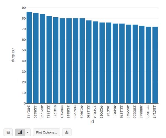
display(scene_graphs_train.degrees.sort(["degree"],ascending=[0]).limit(20))

2_1

Finding most common attributes

"Which object characteristics are the most common?"

from pyspark.sql.functions import explode
# the attributes are sequences: we need to split them;
# explode the attributes in the vertices graph:
explodedAttributes = scene_graphs_train.vertices.select("id", "object_name", explode(scene_graphs_train.vertices.attributes).alias("attribute"))
explodedAttributes.printSchema()
display(explodedAttributes)

Above we see the object-attribute pairs seen in the dataset.

Most used attributes

topAttributes = explodedAttributes.groupBy("attribute")
display(topAttributes.count().sort("count", ascending=False))

2_2

topAttributes = explodedAttributes.groupBy("attribute")
display(topAttributes.count().sort("count", ascending=False))

2_3

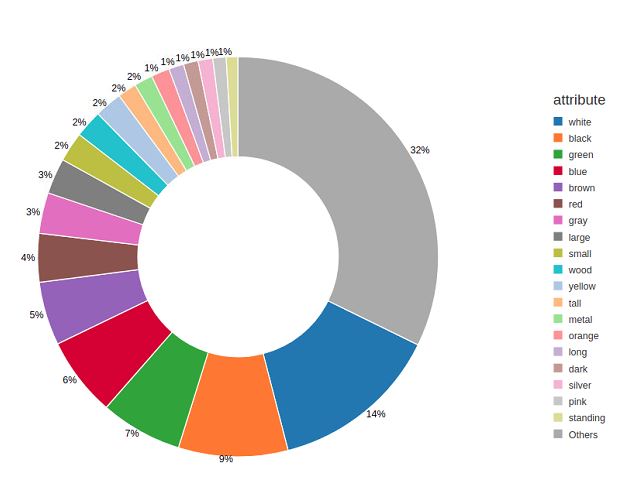
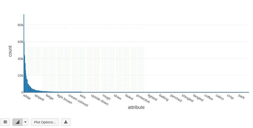
7 out of the top 10 attributes are colors, where white is seen 92659 times, and black 59617 times.
We see a long tail-end distribution with only 68 out of a 617 attributes being seen more than a 1000 times in the dataset, and around 300 attributes are seen less than 100 times (e.g., breakable is seen 15 times, wrist 14 times, and immature 3 times).

Finding most common objects

topObjects = scene_graphs_train.vertices.groupBy("object_name")
topObjects = topObjects.count()
display(topObjects.sort("count", ascending=False))

2_4

display(topObjects.sort("count", ascending=True))

2_5

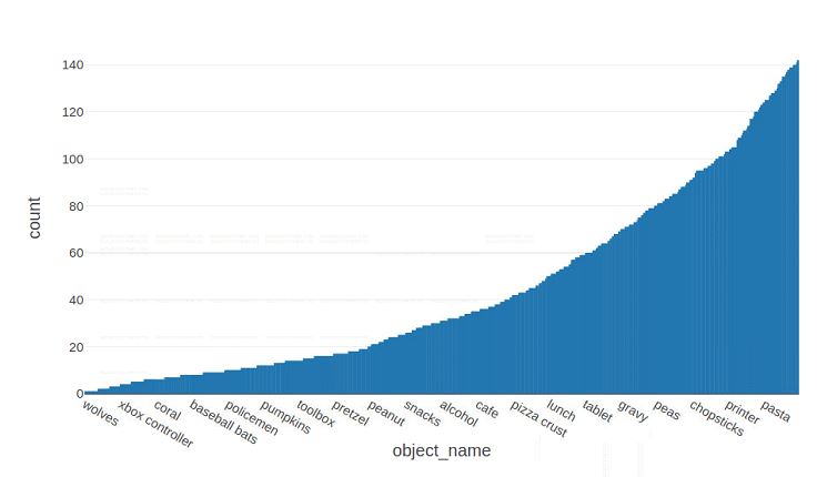
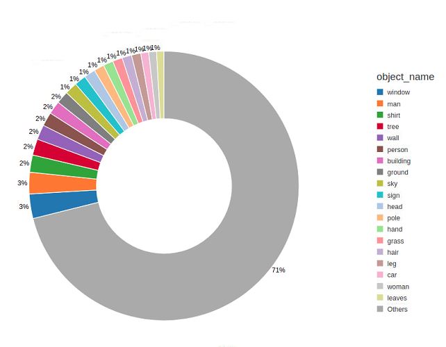
Again, we see that a few object types account for most of the occurrences. Interestingly, man (31370) and person (20218) is seen three and two times more than woman (11355), respectively. Apparently, windows are really important in this dataset, coming out on top with 35907 occurrences.
The top 259 object types are seen more than 1000 times, and after 819 objects are seen less than 100 times.
Looking at the tail-end of the distribution, we see that pikachu is mentioned once, whereas, e.g., wardrobe (5) and robot(8) are rarely seen which was not expected.
The nature of the GQA dataset suggests its general-purpose applicability. However, the skewed object categories distribution shown above implies otherwise.

Finding most common object pairs

"What are the most common two adjacent object categories in the graphs?"

topPairs = scene_graphs_train.edges.groupBy("src_type", "dst_type")
display(topPairs.count().sort("count", ascending=False))

topPairs = scene_graphs_train.edges.groupBy("src_type", "relation_name", "dst_type")
display(topPairs.count().sort("count", ascending=False))

In the tables above, we see that the most common relations reflect spatial properties such as to the right of with windows symmetrically related to each other standing for 2 x 28944 occurrences.
The most common relations are primarily between objects of the same category.
The first 'action'-encoding relation is seen in the 15th most common triple man-wearing-shirt (5254).

Finding most common relations

Could we categorise the edges according to what semantic function they play?
For instance, filtering out all spatial relations (behind, to the left of, etc.).
Suggested categories: spatial, actions, and semantic relations.

topPairs = scene_graphs_train.edges.groupBy("relation_name")
display(topPairs.count().sort("count", ascending=False))

The most common relations are spatial, overwhelmingly, with to the left of and to the right of accounting for 1.7 million occurrences each.
In contrast, the third most common relation on is seen "only" 90804 times. Out of the top 30 relations, 23 are spatial. Common actions can be seen as few times as 28, as in the case of opening.
Some of these relations encode both spatial and actions, such as in sitting on.
This shows some ambiguity in how the relation names are chosen, and how this relates to the attributes, such as sitting, looking, lying, that can also be encoded as object attributes.

Next, we filter out relations that begin with to the, in, on, behind of, or in front of, in order to bring forth more of the non-spatial relations.

# Also possible to do:
# from pyspark.sql.functions import udf
#from pyspark.sql.types import BooleanType

#filtered_df = spark_df.filter(udf(lambda target: target.startswith('good'),
#                                  BooleanType())(spark_df.target))

topPairs = scene_graphs_train.edges.filter("(relation_name NOT LIKE 'to the%') and (relation_name NOT LIKE '%on') and (relation_name NOT LIKE '%in') and (relation_name NOT LIKE '% of')").groupBy("src_type", "relation_name", "dst_type")
display(topPairs.count().sort("count", ascending=False))

2_6

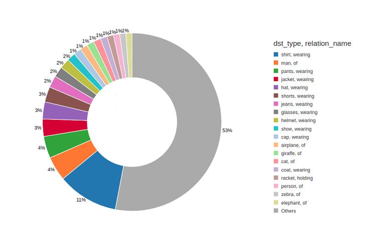
In the pie chart above, we see that once we filter out the most common spatial relations, the remainder is dominated by wearing and the occasional associative of (as in, e.g., head-of-man).
These relations make up almost half of the non-spatial relations.

Finding motifs

scene_graphs_train_without_attributes_graphid = GraphFrame(scene_graphs_train_without_attributes.vertices.select('id', 'object_name'), scene_graphs_train_without_attributes.edges)

motifs = scene_graphs_train_without_attributes_graphid.find("(a)-[ab]->(b); (b)-[bc]->(c)").filter("(a.object_name NOT LIKE b.object_name) and (a.object_name NOT LIKE c.object_name)")

display(motifs)

motifs_sorted = motifs.distinct()
display(motifs_sorted)

motifs_sorted.count()

Find circular motifs, i.e., motifs of type A -> relation_ab -> B -> relation_bc -> C -> relation_ca -> A:

circular_motifs = scene_graphs_train.find("(a)-[ab]->(b); (b)-[bc]->(c); (c)-[ca]->(a)")

display(circular_motifs)

circular_motifs.count()

This gives us 7 million cycles of length 3. However, this is most likely dominated by the most common spatial relations. In the cell below, we filter out these spatial relations and count cycles again.

circular_motifs = scene_graphs_train.find("(a)-[ab]->(b); (b)-[bc]->(c); (c)-[ca]->(a)").filter("(ab.relation_name NOT LIKE 'to the%') and (bc.relation_name NOT LIKE 'to the%') and (ca.relation_name NOT LIKE 'to the%') and (ab.relation_name NOT LIKE '% of') and (bc.relation_name NOT LIKE '% of') and (ca.relation_name NOT LIKE '% of')")

display(circular_motifs.select('ab', 'bc', 'ca'))

circular_motifs.count()

Without the most common spatial relations, we now have a significantly lower amount, 18805, of cycles of length 3.

Find symmetric motifs, i.e., motifs of type A -> relation_ab -> B -> relation_ab -> A:

symmetric_motifs = scene_graphs_train.find("(a)-[ab]->(b); (b)-[ba]->(a)").filter("ab.relation_name LIKE ba.relation_name")

display(symmetric_motifs)

symmetric_motifs.count()

symmetric_motifs = scene_graphs_train.find("(a)-[ab]->(b); (b)-[ba]->(a)").filter("ab.relation_name LIKE ba.relation_name").filter("(ab.relation_name NOT LIKE 'near') and (ab.relation_name NOT LIKE '% of')")

display(symmetric_motifs.select('ab', 'ba'))

symmetric_motifs.count()

The symmetric relations that are spatial behave as expected, and removing the most common ones shows that we have 3693 such symmetric relations.
However, when looking at the filtered symmetric motifs, we can see examples such as 'boy-wearing-boy' and 'hot dog-wrapped in-hot dog'.
These examples of symmetric action relations seem to reflect the expected structure of a scene graph poorly.
We assume that this is either an artefact of the human annotations containing noise or that the sought after denseness of the graphs used describing the images creates these kinds of errors.

Object ranking using PageRank

temp = GraphFrame(scene_graphs_train.vertices.select('graph_id', 'id', 'object_name'), scene_graphs_train.edges)
temp.vertices.write.parquet("/tmp/motif-vertices")
temp.edges.write.parquet("/tmp/motif-edges")

temp = GraphFrame(scene_graphs_val.vertices.select('graph_id', 'id', 'object_name'), scene_graphs_val.edges)#
temp.vertices.write.parquet("/tmp/motif-vertices-val")
temp.edges.write.parquet("/tmp/motif-edges-val")

import org.graphframes.{examples,GraphFrame}

val vertices = sqlContext.read.parquet("/tmp/motif-vertices")
val edges = sqlContext.read.parquet("/tmp/motif-edges")
val rank_graph = GraphFrame(vertices, edges)

import org.graphframes.{examples, GraphFrame}
vertices: org.apache.spark.sql.DataFrame = [graph_id: string, id: string ... 1 more field]
edges: org.apache.spark.sql.DataFrame = [src: string, dst: string ... 3 more fields]
rank_graph: org.graphframes.GraphFrame = GraphFrame(v:[id: string, graph_id: string ... 1 more field], e:[src: string, dst: string ... 3 more fields])

val vertices_val = sqlContext.read.parquet("/tmp/motif-vertices-val")
val edges_val = sqlContext.read.parquet("/tmp/motif-edges-val")
val rank_graph_val = GraphFrame(vertices_val, edges_val)

vertices_val: org.apache.spark.sql.DataFrame = [graph_id: string, id: string ... 1 more field]
edges_val: org.apache.spark.sql.DataFrame = [src: string, dst: string ... 3 more fields]
rank_graph_val: org.graphframes.GraphFrame = GraphFrame(v:[id: string, graph_id: string ... 1 more field], e:[src: string, dst: string ... 3 more fields])

val ranks = rank_graph.pageRank.resetProbability(0.15).tol(0.01).run()
display(ranks.vertices)

#temp = GraphFrame(scene_graphs_train.vertices.select('graph_id', 'id', 'object_name'), scene_graphs_train.edges)

#ranks = temp.pageRank(resetProbability=0.15, tol=0.01)
#display(ranks.vertices)

import org.apache.spark.sql.functions._

val sorted_ranks = ranks.vertices.sort(col("pagerank").desc)
display(sorted_ranks)

val val_graphs_without_attributes = GraphFrame(rank_graph_val.vertices.select("graph_id", "id", "object_name"), rank_graph_val.edges)
val val_ranks = val_graphs_without_attributes.pageRank.resetProbability(0.15).tol(0.01).run()
display(val_ranks.vertices)

val val_sorted_ranks = val_ranks.vertices.sort(col("pagerank").desc)
display(val_sorted_ranks)

val graph_pagerank_sums_objects = ranks.vertices.groupBy("object_name").sum("pagerank")
graph_pagerank_sums_objects.show()

val graph_pagerank_sums_objects_sorted = graph_pagerank_sums_objects.sort(col("sum(pagerank)").desc)

graph_pagerank_sums_objects_sorted: org.apache.spark.sql.Dataset[org.apache.spark.sql.Row] = [object_name: string, sum(pagerank): double]

display(graph_pagerank_sums_objects_sorted)

Here, we see that the summed (accumulated) PageRank per object category reflects each object's number of occurrences (see the topObjects section). At least for the top 10 in this table.
This verifies that the most common objects are highly connected with others in their respective scene graphs.
We, therefore, conclude that they do not necessarily have a high information gain.
A high accumulated PageRank suggests a general nature of objects.

#%scala
val object_count = rank_graph.vertices.groupBy("object_name").count()
display(object_count)

We now sort by name so that we can perform a join.

val topObjects = object_count.sort(col("object_name").desc)
val graph_pagerank_sums_objects_sorted = graph_pagerank_sums_objects.sort(col("object_name").desc)
display(graph_pagerank_sums_objects_sorted)

val graph_pagerank_joined = graph_pagerank_sums_objects_sorted.join(topObjects, "object_name").withColumn("normalize(pagerank)", col("sum(pagerank)") / col("count"))
display(graph_pagerank_joined.sort(col("normalize(pagerank)").desc))

We further normalise the PageRank values, i.e., divide by the number of occurrences per object category in the scenes.
We observe that, in contrast to the accumulated PageRank, the normalised values reflect the uniqueness of object categories: the fewer the occurrences, the higher the normalised PageRank.
For example, televisions occurs only once in the entire dataset. Its corresponding PageRank (accumulated equals normalised in this case) is the highest of all, followed by pizza oven with 9 occurrences.w sort by name so that we can perform a join.

display(graph_pagerank_joined.sort(col("sum(pagerank)").desc).limit(30))

In the above table, we see that the normalised PageRank for the top 30 objects has a different ordering than the summed PageRanks.
For example, pole has the highest normalised PageRank, and the most common category window has a lower value.
An interesting observation is that the objects ground and sky both, relatively, have a significantly lower normalised PageRank, suggesting that a lower PageRank implies a lower semantic information gain. This can be explained by the fact that background objects like sky are rarely the main focus of an image.

val graph_pagerank_sums = ranks.vertices.groupBy("graph_id").sum("pagerank")
display(graph_pagerank_sums)

val graph_val_pagerank_sums = val_ranks.vertices.groupBy("graph_id").sum("pagerank")
display(graph_val_pagerank_sums)

display(graph_val_pagerank_sums.sort(col("sum(pagerank)").desc))

Merging vertices

We use object names (object categories with or without attributes) instead of IDs as vertex identifier to merge all scene graphs (each with its graph_id) into one meta-graph.
This enables us to analyse, e.g., how object types relate to each other in general, and how connected components can be formed based on specific image contexts.
The key intuition is that it could allow us to detect connected components representing scene categories such as traffic or bathroom, i.e., meta-understanding of images as a whole.

merged_vertices = scene_graphs_val.vertices.selectExpr('object_name as id', 'attributes as attributes')
display(merged_vertices)

merged_vertices.count()

merged_vertices = merged_vertices.distinct()
display(merged_vertices)

merged_vertices.count()

We see that there are 22243 unique combinations of objects and attributes.

merged_vertices_without_attributes = merged_vertices.select('id').distinct()
display(merged_vertices_without_attributes)

merged_vertices_without_attributes.count()

merged_edges = scene_graphs_val.edges.selectExpr('src_type as src', 'dst_type as dst', 'relation_name as relation_name')
display(merged_edges)

merged_edges.count()

scene_graphs_merged = GraphFrame(merged_vertices, merged_edges)

# display(scenegraphsmerged.vertices)

display(scene_graphs_merged.edges)

scene_graphs_merged_without_attributes = GraphFrame(merged_vertices_without_attributes, merged_edges)

display(scene_graphs_merged_without_attributes.vertices)

display(scene_graphs_merged_without_attributes.edges)

Computing the Connected Components

Here we compute the connected components of the merged scene graphs (one with the object attributes included and the other without).
Before merging, the connected components should roughly correspond to the number of scene graphs, as they are made up of at least 1 connected component each.
In the merged graphs, we can expect a much smaller set of connected components, and we hypothesize that these could correspond to scene categories (image classes).

sc.setCheckpointDir("/tmp/scene-graph-motifs-connected-components")
connected_components = scene_graphs_merged.connectedComponents()
display(connected_components)

# displays the index of a component for a given object category

components_count = connected_components.groupBy('component')
display(components_count.count().sort("count", ascending=False))

component	count
0.0	22221.0
5.92705486854e11	2.0
1.082331758595e12	1.0
1.88978561028e11	1.0
2.92057776131e11	1.0
8.589934595e9	1.0
4.20906795012e11	1.0
1.090921693187e12	1.0
3.35007449088e11	1.0
8.76173328385e11	1.0
3.60777252879e11	1.0
1.657857376265e12	1.0
2.31928233985e11	1.0
1.279900254215e12	1.0
1.013612281856e12	1.0
1.06515188942e12	1.0
8.50403524616e11	1.0
9.44892805124e11	1.0
1.563368095744e12	1.0
1.700807049221e12	1.0
1.606317768704e12	1.0
1.571958030336e12	1.0

The number of connected components for the merged graph with attributes is 22, with the first component containing almost all instances.

We now run the connected components for the merged meta-graph without the attributes.

connected_components_without_attributes = scene_graphs_merged_without_attributes.connectedComponents()
display(connected_components_without_attributes)

components_count = connected_components_without_attributes.groupBy('component')
display(components_count.count().sort("count", ascending=False))

These results indicate that the merged graph is too dense due to the generic relations (e.g., the spatial relations 'next-to' et al.) connecting all objects into one big chunk.
Removing some of these most occurring relations could show an underlying graph structure that is more interesting.

General discussion

First, we recap the main points of the results of our analysis.

Objects

Interestingly, man (31370) and person (20218) is seen three and two times more than woman (11355), respectively.
The nature of the GQA dataset suggests its general-purpose applicability. However, the skewed object categories distribution shown above implies otherwise.

Attributes

Our analysis of the original dataset shows that a few of the most commonly annotated attributes account for the majority of all annotations.
Most common attributes are colours, black and white being the most common. white is seen 92659 times, and black 59617 times.
We suspect that since the dataset is generated using human annotators, many of the less common annotations, such as attributes occurring less than 100 times, are more error-prone and might have a high noise to label ratio.

Relations

The most common relations are, overwhelmingly, spatial properties with to the left of and to the right of, accounting for 1.7 million occurrences each.
The most common relations are primarily between objects of the same category.
For instance, windows are symmetrically related to each other, making up 2 x 28944 occurrences.
Some of these relations encode both spatial and action relation categories, e.g., sitting on.

PageRank

Our page rank results mainly reflect the number of occurrences of each object category.

To summarize, we see that GQA still has much room for improvement in terms of the distribution of objects and relations.

The analysis can be further deepened by considering the visual information provided in the dataset, i.e., the images.

sds-3.x/ScaDaMaLe