Genomics Analysis with Glow and Spark
Project Members - Karin Stacke - Milda Pocoviciute
Link to video: https://youtu.be/6VMeHixsJ3g
The aim of this notebook is to analyze genomic data in the form of SNPs, and see how different variations of SNPs correlated to ethnicity. This work is inspired by the paper from Huang et al., Genetic differences among ethnic groups (2015), and the notebook https://glow.readthedocs.io/en/latest/_static/notebooks/tertiary/gwas.html.
Problem background
Each person as a unique setup of DNA. The DNA consitst of necleotides, structured as a double helix, where each neucliotide binds to one other. The DNA is split between 23 pairs of chromosomes. There are four different neucliotides, commonly denoted as A, T, C, and G.
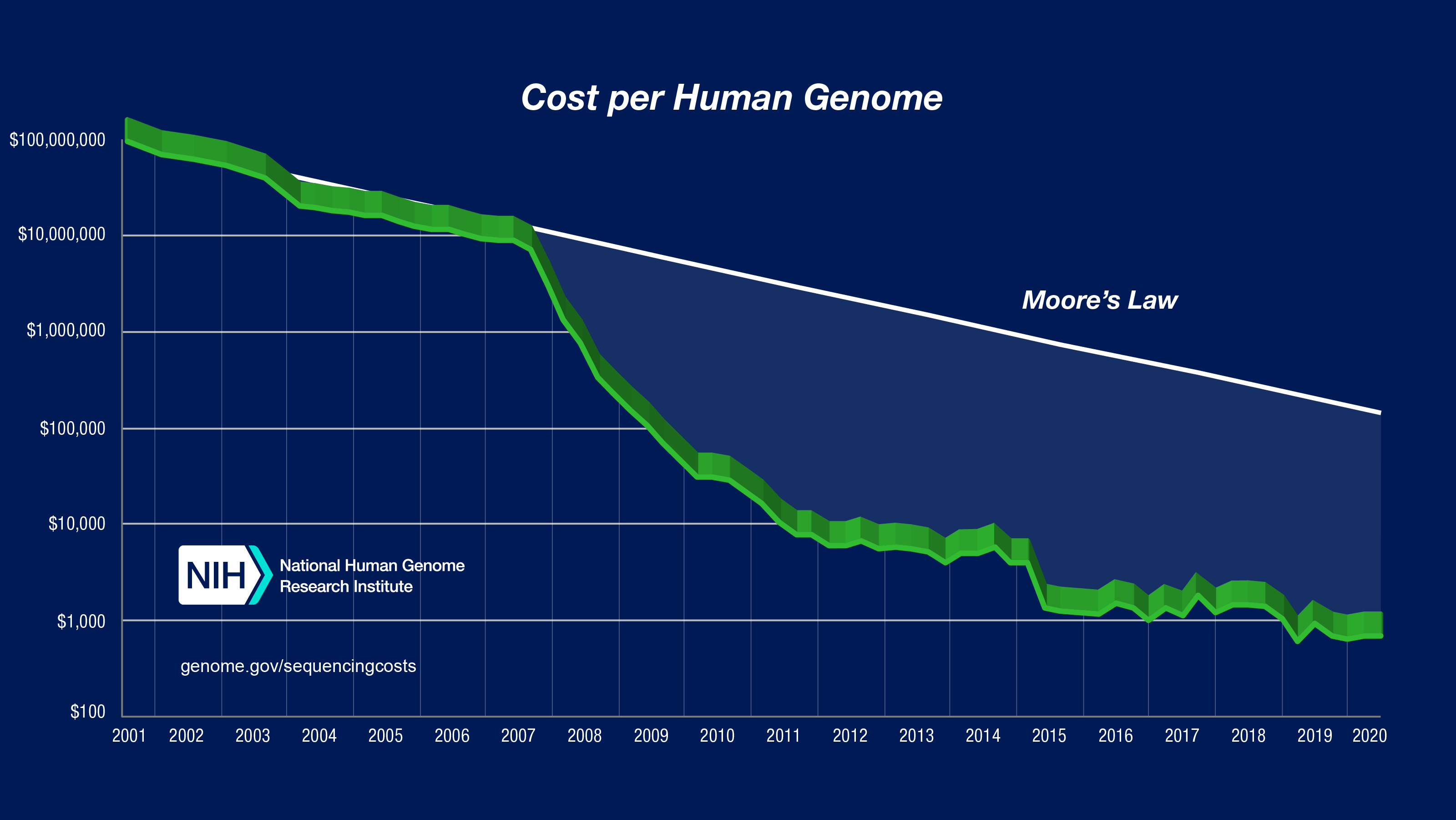
Single nucleotide polymorphisms (SNPs) are the most common genetic variation between individuals. Each SNP represents a variation of a specific neucleotide. For example, a SNP may replace the nucleotide cytosine (C) with the nucleotide thymine (T) in a certain stretch of DNA. The recent sharp decrease in the cost of sequencing a human genome, made it possible to collect and make publically available such datasets for research.
Data
Genomic data is collected from the 1000 Genomes project, with corresponding sample annotations for all individuals in the dataset. For simiplicty, we are only analyzing SNPs assosiated to chromosome 1, however this study can easily be extended to include SNPs from all chromosomes.
The data consists of approximatly 6.5 million SNPs from 2504 subjects.
Method
After reading the data, we filter low quality SNPs. After this operation, we end up with approx. 400'000 SNPs.
By doing a correlation analysis using PCA, we see that different ethnicities cluster together. There is therfore a good reason to suppose that SNPs can be used to predict ethnicity. However, since not all SNPs are correlated to ethnicity, we want to only use the most relevant ones for linear regression analysis.
For each SNPs, we calculate the correlation between the values and ethnicity, and take the SNPs with a higher correlation than a threshold value of 0.6 (or maximum 2000 SNPs).
Using the selected SNPs as features, we do a linear regression analysis. We make some plots.
import matplotlib.pyplot as plt
import numpy as np

from pyspark.sql.functions import array_min, col, monotonically_increasing_id, when, log10
from pyspark.sql.types import StringType
from pyspark.ml.linalg import Vector, Vectors, SparseVector, DenseMatrix
from pyspark.ml.stat import Summarizer
from pyspark.mllib.linalg.distributed import RowMatrix
from pyspark.mllib.util import MLUtils
from pyspark.ml.feature import IndexToString, StringIndexer
from pyspark.ml.feature import OneHotEncoder
from pyspark.sql.functions import col,lit

from dataclasses import dataclass

import mlflow
import glow
glow.register(spark)
# Helper functions

def plot_layout(plot_title, plot_style, xlabel):
  plt.style.use(plot_style) #e.g. ggplot, seaborn-colorblind, print(plt.style.available)
  plt.title(plot_title)
  plt.xlabel(r'${0}$'.format(xlabel))
  plt.gca().spines['right'].set_visible(False)
  plt.gca().spines['top'].set_visible(False)
  plt.gca().yaxis.set_ticks_position('left')
  plt.gca().xaxis.set_ticks_position('bottom')
  plt.tight_layout()

def plot_histogram(df, col, xlabel, xmin, xmax, nbins, plot_title, plot_style, color, vline, out_path):
  plt.close()
  plt.figure()
  bins = np.linspace(xmin, xmax, nbins)
  df = df.toPandas()
  plt.hist(df[col], bins, alpha=1, color=color)
  if vline:
    plt.axvline(x=vline, linestyle='dashed', linewidth=2.0, color='black')
  plot_layout(plot_title, plot_style, xlabel)
  plt.savefig(out_path)
  plt.show()

def calculate_pval_bonferroni_cutoff(df, cutoff=0.05):
  bonferroni_p =  cutoff / df.count()
  return bonferroni_p

def get_sample_info(vcf_df, sample_metadata_df):
  """
  get sample IDs from VCF dataframe, index them, then join to sample metadata dataframe
  """
  sample_id_list = vcf_df.limit(1).select("genotypes.sampleId").collect()[0].__getitem__("sampleId")
  sample_id_indexed = spark.createDataFrame(sample_id_list, StringType()). \
                            coalesce(1). \
                            withColumnRenamed("value", "Sample"). \
                            withColumn("index", monotonically_increasing_id())
  sample_id_annotated = sample_id_indexed.join(sample_metadata_df, "Sample")
  return sample_id_annotated
# Paths to store/find data.
# Since a lot of the processing takes a long time, we store intermediate results.
vcf_path = "dbfs:///datasets/sds/genomics/ALL.chr1.phase3_shapeit2_mvncall_integrated_v5a.20130502.genotypes.vcf.gz"
delta_silver_path = "/mnt/gwas_test/snps.delta"

gwas_results_path = "/mnt/gwas_test/gwas_results.delta"
phenotype_path = "/databricks-datasets/genomics/1000G/phenotypes.normalized"
sample_info_path = "/databricks-datasets/genomics/1000G/samples/populations_1000_genomes_samples.csv"

principal_components_path = "/dbfs/datasets/sds/genomics/pcs.delta"
hwe_path = "dbfs:///datasets/sds/genomics/hwe.delta"
vectorized_path = "dbfs:///datasets/sds/genomics/vectorized.delta"
delta_gold_path = "dbfs:///datasets/sds/genomics/snps.qced.delta.delta"
The data used was dowloaded from ftp://ftp.1000genomes.ebi.ac.uk/vol1/ftp/release/20130502/ALL.chr1.phase3shapeit2mvncallintegratedv5a.20130502.genotypes.vcf.gz
wget ftp://ftp.1000genomes.ebi.ac.uk/vol1/ftp/release/20130502/ALL.chr1.phase3_shapeit2_mvncall_integrated_v5a.20130502.genotypes.vcf.gz
Read data
The data is read using the Glow, an open-source library for working with genomics data in a scallable way. It is inlcuded when enabling "Databricks Runtime for Genomics", allowing easy read of genomic-specific file formats, and other helper methods.
Load and view the vcf files. The info fields are combined to one column.
vcf_view_unsplit = spark.read.format("vcf"). \
   option("flattenInfoFields", "false"). \
   load(vcf_path)

display(vcf_view_unsplit.withColumn("genotypes", col("genotypes")[1]))
In the dataframe above, we see that we have columns named "referenceAllele" and "alternateAlleles". The data so called variations, i.e., genetic sequences which are different between two individuals. The difference may appear differently, and each difference is called an allele. In the data, we have reference genomes, and the alternate alleles are all the variations at a specific position which is found amoung the analyzed subjects.
We do not want multiple alternative allelels in one row, so we split them using the split_miltiallelics function from Glow.
vcf_view = glow.transform("split_multiallelics", vcf_view_unsplit)
display(vcf_view.withColumn("genotypes", col("genotypes")[1]))
We now save our modified dataframe in the Delta format (which compared to VCF is more user friendly). At the same time, we calulcate som neccessary statistics, which we will use later, using the Glow functions call_summary_stats and hardy_weinberg.
# NOTE - this takes approx 2 hours

vcf_view.selectExpr("*", "expand_struct(call_summary_stats(genotypes))", "expand_struct(hardy_weinberg(genotypes))"). \
   write. \
   mode("overwrite"). \
   format("delta"). \
   save(delta_silver_path)
The statistics we calculated, as well as the Hardy-Weinberg equilibrium p-values (which basically denotes the probability of a given allele is probable to be true or may be a reading mistake), are used to filter out low quality SNPs.
We read the saved dataframe, and filter the dataframe.
# Hyper paramters
allele_freq_cutoff = 0.05
num_pcs = 5 #number of principal components
hwe = spark.read.format("delta"). \
                 load(delta_silver_path). \
                 where((col("alleleFrequencies").getItem(0) >= allele_freq_cutoff) &
                       (col("alleleFrequencies").getItem(0) <= (1.0 - allele_freq_cutoff))). \
                 withColumn("log10pValueHwe", when(col("pValueHwe") == 0, 26).otherwise(-log10(col("pValueHwe"))))

hwe.write. \
   mode("overwrite"). \
   format("delta").save(hwe_path)

hwe = spark.read.format('delta').load(hwe_path)
hwe_cutoff = calculate_pval_bonferroni_cutoff(hwe)
Filter and save new dataframe, only alleles with in the frequency band, and where the Hardy-Weiburg value is higher than cutoff.
spark.read.format("delta"). \
   load(hwe_path). \
   where((col("alleleFrequencies").getItem(0) >= allele_freq_cutoff) &
         (col("alleleFrequencies").getItem(0) <= (1.0 - allele_freq_cutoff)) &
         (col("pValueHwe") >= hwe_cutoff)). \
   write. \
   mode("overwrite"). \
   format("delta"). \
   save(delta_gold_path)
# We saved the results to disc and here we jus tload them as the above computation takes a lot of time
hwe_filtered = spark.read.format('delta').load(delta_gold_path)
PCA
We perform a PCA analysis for data exploration purposes.
vectorized = spark.read.format("delta"). \
                        load(delta_gold_path). \
                        selectExpr("array_to_sparse_vector(genotype_states(genotypes)) as features"). \
                        cache()

vectorized.write. \
   mode("overwrite"). \
   format("delta").save("dbfs:///datasets/sds/genomics/vectorized.delta")

# We saved the results to disc and here we jus tload them as the above computation takes a lot of time
vectorized = spark.read.format('delta').load(vectorized_path)
display(vectorized)
# Note - takes approx 30 min

matrix = RowMatrix(MLUtils.convertVectorColumnsFromML(vectorized, "features").rdd.map(lambda x: x.features))
pcs = matrix.computeSVD(num_pcs)
@dataclass()
class Covariates:
    covariates: DenseMatrix

spark.createDataFrame([Covariates(pcs.V.asML())]). \
      write. \
      format("delta"). \
      save(principal_components_path)
pcs_df = spark.createDataFrame(pcs.V.toArray().tolist(), ["pc" + str(i) for i in range(num_pcs)])

display(pcs_df)

pcs_df.coalesce(1).write.format("com.databricks.spark.csv").option("header", "true").save("dbfs:///datasets/sds/genomics/pcs_df.csv")
# Read already caluclated pca
pcs_df = spark.read.format('csv').load("dbfs:///datasets/sds/genomics/pcs_df.csv")
display(pcs_df)
**Read sample metadata and add to PCA components **
We load the subject meta data (which includes information about ethnicity).
sample_metadata = spark.read.option("header", True).csv(sample_info_path)
sample_info = get_sample_info(vcf_view, sample_metadata)

sample_count = sample_info.count()

pcs_indexed = pcs_df.coalesce(1).withColumn("index", monotonically_increasing_id())
pcs_with_samples = pcs_indexed.join(sample_info, "index")
View 1st and 2nd principal component
display(pcs_with_samples)

We see that there there are some clustering based on ethnicity, showing that it could be possible to tell ethnicity from the SNP information of a subject.
Replication of the paper "Genetic differences among ethnic groups", Huang et al. https://bmcgenomics.biomedcentral.com/articles/10.1186/s12864-015-2328-0
Originally, we had approx. 6.5 milj genetic variations, from 2500 individuals. We first did a quality control by filtering only alleles which occur frequently enough, and those above the Hardy-Weinberg P value cutoff.
Since we still have over 400 000 variations, we need to filter further and only keep the SNPs that have significant correlation to ethnicity. We experiment with several different sizes of the final data set.
Here we read the dataset that contains the population information and encode it for regression
# Read sample information
sample_metadata = spark.read.option("header", True).csv(sample_info_path)
sample_info = get_sample_info(vcf_view, sample_metadata)

sample_count = sample_info.count()

mlflow.log_param("number of samples", sample_count)
From the plot below we can see that our data set is not balanced as we have more samples from african ethnicity than any other. We decided not to balance the data and see if this would have obvious negative impact on our results.
display(sample_info)

# One hot encoding of the labels
from pyspark.ml.feature import IndexToString, StringIndexer
from pyspark.ml.feature import OneHotEncoder

# indexer = StringIndexer(inputCol="Population", outputCol="Population_index")
indexer = StringIndexer(inputCol="super_population", outputCol="Population_index")
model = indexer.fit(sample_info)
indexed = model.transform(sample_info)

# indexed.select("Population", "Population_index").distinct().show(30)

encoder = OneHotEncoder(inputCols=["Population_index"],
                        outputCols=["population_onehot"])
model = encoder.fit(indexed)
encoded = model.transform(indexed)
encoded.show()
Filtering of SNPs based on chi-squared test
According to Tao Huang et al. (2015), 85 % of SNPs are the same in all human populations, hence we will apply chi-squared based feature selection to try to identify the approximately 15 % of SNPs that are population-specific. We decided to test our classifiers with several sizes of the feature vectors: * all 416,005 available SNPs from Chromosome 1 * most relevant 200,000 SNPs * most relevant 20,000 SNPs * most relevant 2,000 SNPs * most relevant 1,000 SNPs * most relevant 100 SNPs * most relevant 50 SNPs
This would give us a better understanding if the ChiSqSelector is appropriate method for selecting the features in genomics. We aklowedge that Tao Huang et al. (2015) used different metric based on chi-squared distribution, but ChiSqSelector is the closest already implemented method in spark that we could find.
In order to use ChiSqSelector from pyspark.ml.feature, we first need to format the data into a sparce feature vectors and numeric corresponding label.
# Load earlier-filtered data
delta_gold_path = "dbfs:///datasets/sds/genomics/snps.qced.delta.delta"
hwe_filtered = spark.read.format('delta').load(delta_gold_path)
vectorized_2 = hwe_filtered.select(glow.genotype_states('genotypes').alias('states')).collect()
vectorized_df = spark.createDataFrame(vectorized_2)
display(vectorized_df)
We use monotonicallyincreasingid, poseexplode and collect_list methods to achieve the required format of the data:
# Add a column that indicates to which SNP the states belong and then explode SNPs
from pyspark.sql.functions import monotonically_increasing_id
from pyspark.sql.functions import explode, posexplode
from pyspark.sql.functions import col, concat, desc, first, lit, row_number, collect_list

vec_df_dummy = vectorized_df.withColumn("SNP", monotonically_increasing_id())
#vec_exploded_states = vec_df_dummy.withColumn("expanded_states", explode("states"))
vec_exploded_states = vec_df_dummy.select("SNP",posexplode("states"))
vec_exploded_states = vec_exploded_states.withColumnRenamed("pos", "subjectID")
vec_exploded_states = vec_exploded_states.withColumnRenamed("col", "expandedState")
features_df = vec_exploded_states.groupBy("subjectID").agg(collect_list("expandedState").alias("Features"))
features_df = features_df.join(encoded, features_df.subjectID == encoded.index).select("Features","Population_index", "population_onehot")
features_df.show()
Finally, Glow utility function arraytosparse_vector is used to convert the dense feature vectors into sparse vectors
features_df = features_df.selectExpr("array_to_sparse_vector(Features) as features_sparse","Population_index", "population_onehot")
features_df.show()
Fitting ChiSqSelector
As the computation time of ChiSqSelector takes roughly 3 hours for each subset of features, we are saving them to disc.
feature_selection_200_000 = "dbfs:///datasets/sds/genomics/selected_feat_200_000.delta"
from pyspark.ml.feature import ChiSqSelector
# selector = ChiSqSelector(featuresCol='features_sparse', outputCol='ChiSq',labelCol='Population_index', numTopFeatures = 200000)
# selected_feat_200_000 = selector.fit(features_df).transform(features_df)
# selected_feat_200_000.write.format("delta").save(feature_selection_200_000)
selected_feat_200_000 = spark.read.format('delta').load(feature_selection_200_000)
feature_selection_20_000 = "dbfs:///datasets/sds/genomics/selected_feat_20_000.delta"
# selector = ChiSqSelector(featuresCol='features_sparse', outputCol='ChiSq',labelCol='Population_index', numTopFeatures = 20000)
# selected_feat_20_000 = selector.fit(features_df).transform(features_df)
# selected_feat_20_000.write.format("delta").save(feature_selection_20_000)
selected_feat_20_000 = spark.read.format('delta').load(feature_selection_20_000)
feature_selection_2000 = "dbfs:///datasets/sds/genomics/selected_feat_2000.delta"
# from pyspark.ml.feature import ChiSqSelector
# selector = ChiSqSelector(featuresCol='features_sparse', outputCol='ChiSq',labelCol='Population_index', numTopFeatures = 2000)
# selected_feat_2000 = selector.fit(features_df).transform(features_df)
# selected_feat_2000.write.format("delta").save(feature_selection_2000)

selected_feat_2000 = spark.read.format('delta').load(feature_selection_2000)
selected_feat_2000.show()
feature_selection_results_1000 = "dbfs:///datasets/sds/genomics/selected_feat_1000.delta"
# selector = ChiSqSelector(featuresCol='features_sparse', outputCol='ChiSq',labelCol='Population_index', numTopFeatures = 1000)
# selected_feat_1000 = selector.fit(features_df).transform(features_df)
# selected_feat_1000.write.format("delta").save(feature_selection_results_1000)
#result = selector.fit(features_df).transform(features_df)
selected_feat_1000 = spark.read.format('delta').load(feature_selection_results_1000)
feature_selection_results_100 = "dbfs:///datasets/sds/genomics/selected_feat_100.delta"
# selector = ChiSqSelector(featuresCol='features_sparse', outputCol='ChiSq',labelCol='Population_index', numTopFeatures = 100)
# selected_feat_100 = selector.fit(features_df).transform(features_df)
# selected_feat_100.write.format("delta").save(feature_selection_results_100)
#result = selector.fit(features_df).transform(features_df)
selected_feat_100 = spark.read.format('delta').load(feature_selection_results_100)
feature_selection_50 = "dbfs:///datasets/sds/genomics/selected_feat_50.delta"
# selector = ChiSqSelector(featuresCol='features_sparse', outputCol='ChiSq',labelCol='Population_index', numTopFeatures = 50)
# selected_feat_50 = selector.fit(features_df).transform(features_df)
# selected_feat_50.write.format("delta").save(feature_selection_50)
selected_feat_50 = spark.read.format('delta').load(feature_selection_50)
Train logistic regression and random forest models
The code below implements a loop over datasets with different number of SNPs, test-train split and fitting of logistic regression and random forest models. The performance is measured in accuracy.
from pyspark.ml.classification import LogisticRegression
from pyspark.ml.evaluation import MulticlassClassificationEvaluator
from pyspark.ml.classification import RandomForestClassifier

def fit_ML_model(trainSet,testSet, model_in):

  # Train model.
  model = model_in.fit(trainSet)

  # Make predictions.
  predictions = model.transform(testSet)

  # Evaluate the classifier based on accuracy
  evaluator = MulticlassClassificationEvaluator(
      labelCol="Population_index", predictionCol="prediction", metricName="accuracy")
  accuracy = evaluator.evaluate(predictions)
  return accuracy


rf = RandomForestClassifier(labelCol="Population_index", featuresCol="final_features", numTrees=20)
lr = LogisticRegression(featuresCol="final_features", labelCol="Population_index", maxIter=100)

acc_rf = []
acc_lr = []

# Run the models on full features set (without ChiSqSelector)
features_ready = selected_feat_2000.selectExpr("features_sparse as final_features","Population_index")
trainSet, testSet = features_ready.randomSplit((0.8, 0.2), seed=123)
acc_rf.append(fit_ML_model(trainSet, testSet, rf))
acc_lr.append(fit_ML_model(trainSet, testSet, lr))

# Run the models on selected features by ChiSqSelector
for data_item in [selected_feat_200_000, selected_feat_20_000, selected_feat_2000, selected_feat_1000, selected_feat_100, selected_feat_50]:
    # Work around for the bug in ChiSqSelector - otherwise does not work with the random forest model
    #ChiSqSelector has a bug that it formats data in a way that RandomForest does not accept. We found this work around to work. Bug reported in https://stackoverflow.com/questions/46269275/spark-ml-issue-in-training-after-using-chisqselector-for-feature-selection
    features_ready = data_item.select(glow.vector_to_array('ChiSq').alias('features_dense'), "Population_index", "ChiSq")
    features_ready = features_ready.selectExpr("array_to_sparse_vector(features_dense) as final_features","Population_index")
    trainSet, testSet = features_ready.randomSplit((0.8, 0.2), seed=123)
    acc_rf.append(fit_ML_model(trainSet, testSet, rf))
    acc_lr.append(fit_ML_model(trainSet, testSet, lr))
import matplotlib.pyplot as plt

rf_plot = plt.scatter(x=['all_feat', '200,000', '20,000', '2,000', '1,000', '100', '50'], y=acc_rf, c='r')
lf_plot = plt.scatter(x=['all_feat', '200,000', '20,000', '2,000', '1,000', '100', '50'], y=acc_lr, c='b')
plt.xlabel("Number of features")
plt.ylabel("Accuracy")
plt.legend((rf_plot, lf_plot),
           ('Random forest', 'Logistic regression'),
           scatterpoints=1,
           bbox_to_anchor=(1.5, 1),
           ncol=1,
           fontsize=12)
plt.show()

The plot above shows the accuracy of random forest and logistic regression classifiers on predicting the ethnicity from prepared SNPs. Both classifiers preformed much better than random guessing, hence the ethnicity information is clearly encoded in SNPs. The logistic regression consistently outperformed random forest and reached accuracy over 90 %. We can also see that random forest was sensitive to the feature selection and it's performance droped once fewer that the all available SNPs (416,005 SNPs) were used. In contrast, logistic regression performed equally well with half of the available features (200,000 SNPs). This indicates that having well-tuned classifier and an appropriate feature selector allows us to reduce the required number of features dramatically without compromising the performance.
The work could be improved by testing other ways of selecting the relevant SNPs, tuning the hyperparameters in a grid-search manner, building confidence intervals based on bootstrapping or cross-validation and testing other types of classifiers.