ScaDaMaLe Course site and book

Fundamental Matrix

Group members: Linn Öström, Patrik Persson, Johan Oxenstierna, and Alexander Dürr

Link to our video explaining the 1) theory, 2) preprocessing the dataset, 3) algorithm and 4) results https://drive.google.com/drive/folders/1zEWj6JsJEUu9f8Q5Xy_avwxQ3yJ9oI7Z?usp=sharing

alternatively: https://youtu.be/eJ2LDtNad08

Problem formulation

A common problem in computer vision is estimating the fundamental matrix based on a image pair. The fundamental matrix relates corresponding points in stereo geometry, and is useful as a pre-processing step for example when one wants to perform reconstruction of a captured scene. In this small project we use a scalable distributed algorithm to compute fundamental matrices between a large set of images.

Short theory section

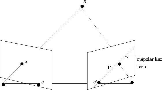
Assume that we want to link points in some image taken by camera $P_1$ to points in an image taken by another camera $P_2$ . Let $x_i$ and $x_i'$ denote the projections of global point $X_i$ onto the cameras $P_1$ and $P_2$ , respectivly. Then the points are related as follows

$\begin{cases}\lambda_i x_i = P_1X_i \\ \lambda_i' x_i' = P_2X_i \end{cases} \Leftrightarrow \quad \begin{cases}\lambda_i x_i = P_1HH^{-1}X_i \\ \lambda_i' x_i' = P_2HH^{-1}X_i \end{cases} \Leftrightarrow \quad \begin{cases}\lambda_i x_i = \tilde{P_1}\tilde{X_i} \\ \lambda_i' x_i' = \tilde{P_2}\tilde{X_i} \end{cases}$

where $\lambda, \lambda'$ are scale factors. Since we always can apply a projective transformation $H$ to set one of the cameras to $P_1 = [I \quad 0]$ and the other to some $P_2 = [A \quad t]$ we can parametrize the global point $X_i$ by $X_i(\lambda) = [\lambda x_i \quad 1]^T$ . Thus the projected point onto camera $P_2$ is represented by the line $P_2X_i(\lambda) = \lambda Ax_i + t$ . This line is called the epipolar line to the point $x_i$ in epipolar geomtry, and descirbes how the point $x_i$ in image 1 is related to points on in image 2. Since all scene points that can project to $x_i$ are on the viewing ray, all points in the second image that can correspond $x_i$ have to be on the epipolar line. This condition is called the epipolar constraint.

plot

Taking two points on this line (one of them being $e'$ using $\lambda = 0$ ), (add what is e_2) we can derive an expression of this line $\ell$ , as any point x on the line $\ell$ must fulfill $\ell^Tx = 0$ . Thus the line is thus given by

$\ell = t \times (Ax +t ) = t \times (Ax) = e' \times Ax_i.\\$

Let $F = e' \times A$ , this is called the fundamental matrix. The fundamental matrix thus is a mathematical formulation which links points in image 1 to lines in image 2 (and vice versa). If $x'$ corresponds to $x$ then the epipolar constraint can be written

$x'^T\ell = x'^T F x = 0$

F is a 3x 3 matrix with 9 entiers and has 7 degrees of freedom. It can be estimated using 7 points using the 7-point algorithm.

Before we have assumed the the correspndeces between points in the imagaes are known, however these are found by first extracting features in the images using some form of feature extractor (e.g. SIFT) and subsequently finding matches using some mathcing criterion/algorithm (e.g. using Lowes criterion or in our case FLANN based matcher)

SIFT

Scale-invariant feature transform (SIFT) is a feature detection algorithm which detect and describe local features in images, see examples of detected SIFT features in the two images (a) and (b). SIFT finds local features present in the image and compute desriptors and locations of these features. Next we need to link the features present in image 1 to the features in image 2, which can be done using e.g. a FLANN (Fast Library for Approximate Nearest Neighbors) based matcher. In short the features in the images are compared and the matches are found using a nearest neighbor search. After a matching algorithm is used we have correspandence between the detected points in image 1 and image 2, see example in image (c) below. Note that there is still a high probaility that some of these matches are incorrect.

RANSAC

Some matches found by the FLANN may be incorrect, and a common robust method used for reducing the influence of these outliers in the estimation of F is RANSAC (RANdom SAmpling Consensus). In short, it relies on the fact that the inliers will tend to a consesus regarding the correct estimation, whereas the outlier estimation will show greater variation. By sampling random sets of points with size corresponding to the degrees of freedom of the model, calculating their corresponding estimations, and grouping all estimations with a difference below a set threshold, the largest consesus group is found. This set is then lastly used for the final estimate of F.

For a more joyful presentation of the theory, listed to The Fundamental Matrix Song! (link)

OpenCV is an well-known open-source library for computer vision, machine learning, and image processing tasks. In this project we will use it for feature extraction (SIFT), feature matching (FLANN) and the estimation of the fundamental matrix (using the 7-point algorithm). Let us install opencv

install opencv-python

Also we need to download a dataset that we can work with, this dataset is collected by Carl Olsson from LTH. This is achieved by the bash shell script below. The dataset is placed in the /tmp folder using the -P "prefix"

rm -r /tmp/0019
rm -r /tmp/eglise_int1.zip

wget -P /tmp vision.maths.lth.se/calledataset/eglise_int/eglise_int1.zip
unzip /tmp/eglise_int1.zip -d /tmp/0019/
rm -r /tmp/eglise_int1.zip

rm -r /tmp/eglise_int2.zip

wget -P /tmp vision.maths.lth.se/calledataset/eglise_int/eglise_int2.zip
unzip /tmp/eglise_int2.zip -d /tmp/0019/
rm -r /tmp/eglise_int2.zip

rm -r /tmp/eglise_int3.zip

wget -P /tmp vision.maths.lth.se/calledataset/eglise_int/eglise_int3.zip
unzip /tmp/eglise_int3.zip -d /tmp/0019/
rm -r /tmp/eglise_int3.zip

cd /tmp/0019/
for f in *; do mv "$f" "eglise_$f"; done
cd /databricks/driver

# for an experiment to detect if images from an unrelated scene are not matched to pictures from another scene
%sh
rm -r /tmp/gbg.zip

wget -P /tmp vision.maths.lth.se/calledataset/gbg/gbg.zip
unzip /tmp/gbg.zip -d /tmp/0019/
rm -r /tmp/gbg.zip

import sys.process._

//"wget -P /tmp vision.maths.lth.se/calledataset/door/door.zip" !!
//"unzip /tmp/door.zip -d /tmp/door/"!!

//move downloaded dataset to dbfs

val localpath="file:/tmp/0019/"

dbutils.fs.rm("dbfs:/datasets/0019/mixedimages", true)  // the boolean is for recursive rm

dbutils.fs.mkdirs("dbfs:/datasets/0019/mixedimages")

dbutils.fs.cp(localpath, "dbfs:/datasets/0019/mixedimages", true)

import sys.process._
localpath: String = file:/tmp/0019/
res5: Boolean = true

rm -r /tmp/0019

display(dbutils.fs.ls("dbfs:/datasets/0019/mixedimages"))

#Loading one image from the dataset for testing

import numpy as np
import cv2
import matplotlib.pyplot as plt

def plot_img(figtitle,img):

  #create figure with std size
  fig = plt.figure(figtitle, figsize=(10, 5))

  plt.imshow(img)

  display(plt.show())

img1 = cv2.imread("/dbfs/datasets/0019/mixedimages/eglise_DSC_0133.JPG")
#img2 = cv2.imread("/dbfs/datasets/0019/mixedimages/DSC_0133.JPG")

plot_img("eglise", img1)
#plot_img("gbg", img2)

ls /dbfs/datasets/0019/mixedimages/eglise_DSC_0133.JPG

Read Image Dataset

import glob
import numpy as np
import cv2
import os

dataset_path  = "/dbfs/datasets/0019/mixedimages/"

#get all filenames in folder
files = glob.glob(os.path.join(dataset_path,"*.JPG"))

dataset = []

#load all images names
for i, file in enumerate(files): # Alex: changed
  # Load an color image
  #img = cv2.imread(file)

  #add image and image name as a tupel to the list
  dataset.append((file))
  if i >= 150: # Alex: changed
    break

Define maps

import glob
import numpy as np
import cv2
import matplotlib.pyplot as plt

max_features = 1000

def plot_img(figtitle,s):

  img = cv2.imread(s)

  #create figure with std size
  fig = plt.figure(figtitle, figsize=(10, 5))

  plt.imshow(img)

  display(plt.show())


def extract_features(s):
  """
  """
  # Here we load the images on the executor from dbfs into memory
  img = cv2.imread(s)

  #convert to gray scale
  gray= cv2.cvtColor(img,cv2.COLOR_BGR2GRAY)

  sift = cv2.SIFT_create(max_features)

  #extract sift features and descriptors
  kp, des = sift.detectAndCompute(gray, None)

  #convert keypoint class to list of feature locations (for serialization)
  points=[]
  for i in range(len(kp)):
    points.append(kp[i].pt)

  #return a tuple of image name, feature points, descriptors, called a feature tuple
  return (s, points, des)

def estimate_fundamental_matrix(s):
  """
  """

  # s[0] is a feature tuple for the first image, s[1] is the same for the second image
  a = s[0]
  b = s[1]

  # unpacks the tuples
  name1, kp1, desc1 = a
  name2, kp2, desc2 = b

  # Create FLANN matcher object
  FLANN_INDEX_KDTREE = 0
  indexParams = dict(algorithm=FLANN_INDEX_KDTREE,
                   trees=5)
  searchParams = dict(checks=50)
  flann = cv2.FlannBasedMatcher(indexParams,
                              searchParams)

  # matches the descriptors, for each query descriptor it finds the two best matches among the train descriptors
  matches = flann.knnMatch(desc1, desc2, k=2)

  goodMatches = []
  pts1 = []
  pts2 = []

  # compares the best with the second best match and only adds those where the best match is significantly better than the next best.
  for i,(m,n) in enumerate(matches):
    if m.distance < 0.8*n.distance:
        goodMatches.append([m.queryIdx, m.trainIdx])
        pts2.append(kp2[m.trainIdx])
        pts1.append(kp1[m.queryIdx])

  pts1 = np.array(pts1, dtype=np.float32)
  pts2 = np.array(pts2, dtype=np.float32)

  # finds the fundamental matrix using ransac:
  # selects minimal sub-set of the matches,
  # estimates the fundamental matrix,
  # checks how many of the matches satisfy the epipolar geometry (the inlier set)
  # iterates this for a number of iterations,
  # returns the fundamental matrix and mask with the largest number of inliers.
  F, mask = cv2.findFundamentalMat(pts1, pts2, cv2.FM_RANSAC)

  inlier_matches = []

  # removes all matches that are not inliers
  if mask is not None:  
    for i, el in enumerate(mask):
      if el == 1:
        inlier_matches.append(goodMatches[i])

  # returns a tuple containing the feature tuple of image one and image two, the fundamental matrix and the inlier matches
  return (a, b, F, inlier_matches)

def display_data(data):
  for el in data:

    print(el[2])

    print("#######################################################")

Perform Calculations

# creates an rdd from the loaded images (im_name)
rdd = sc.parallelize(dataset,20)
print("num partitions: ",rdd.getNumPartitions())

# applys the feature extraction to the images
rdd_features = rdd.map(extract_features) # Alex: we could leave the name but remove the image in a and b
print("num partitions: ",rdd_features.getNumPartitions())

# forms pairs of images by applying the cartisian product and filtering away the identity pair
rdd_pairs = rdd_features.cartesian(rdd_features).filter(lambda s: s[0][0] != s[1][0])
print("num partitions: ",rdd_pairs.getNumPartitions())

# applys the fundamental matrix estimation function on the pairs formed in the previous step and filters away all pairs with a low inlier set.
rdd_fundamental_matrix = rdd_pairs.map(estimate_fundamental_matrix).filter(lambda s: len(s[3]) > 50)
print("num partitions: ",rdd_fundamental_matrix.getNumPartitions())

# collects the result from the nodes
data = rdd_fundamental_matrix.collect()

# displays the fundamental matrices
display_data(data)

Results

Time complexity of our algorithm
Visualizing epipolar lines
Visualizing matching points

Now we have computed the fundamental matrices, let us have a look at them by present the epipolar lines.

import random

def drawlines(img1,img2,lines,pts1,pts2):
  #from opencv tutorial
    ''' img1 - image on which we draw the epilines for the points in img2
        lines - corresponding epilines '''
    r,c,_ = img1.shape
    for r,pt1,pt2 in zip(lines,pts1,pts2):
        color = tuple(np.random.randint(0,255,3).tolist())
        x0,y0 = map(int, [0, -r[2]/r[1] ])
        x1,y1 = map(int, [c, -(r[2]+r[0]*c)/r[1] ])
        img1 = cv2.line(img1, (x0,y0), (x1,y1), color,3)
        img1 = cv2.circle(img1,tuple(pt1),10,color,-1)
        img2 = cv2.circle(img2,tuple(pt2),10,color,-1)
    return img1,img2

# draws a random subset of the data
sampling = random.choices(data, k=4)

#plotts the inlier features in the first image and the corresponding epipolar lines in the second image
i = 0
fig, axs = plt.subplots(1, 8, figsize=(25, 5))
for el in sampling:

  a, b, F, matches = el;

  if F is None:
    continue

  name1, kp1, desc1 = a
  name2, kp2, desc2 = b
  im1 = cv2.imread(name1)
  im2 = cv2.imread(name2)

  pts1 = []
  pts2 = []

  for m in matches:
    pts1.append(kp1[m[0]]);
    pts2.append(kp2[m[1]]);

  pts1 = np.array(pts1, dtype=np.float32)
  pts2 = np.array(pts2, dtype=np.float32)

  lines1 = cv2.computeCorrespondEpilines(pts2.reshape(-1,1,2), 2, F)
  lines1 = lines1.reshape(-1,3)

  img1, img2 = drawlines(im1,im2,lines1,pts1,pts2)

  axs[i].imshow(img2), axs[i].set_title('Image pair '+str(i+1)+': Features')
  axs[i+1].imshow(img1), axs[i+1].set_title('Image pair '+str(i+1)+': Epipolar lines')

  i += 2
  #plt.subplot(121),plt.imshow(img1), plt.title('Epipolar lines')
  #plt.subplot(122),plt.imshow(img2), plt.title('Points')
display(plt.show())

plot

Present Matches

import random

# draws a random subset of the data
sampling = random.choices(data, k=4)

j = 0
fig, axs = plt.subplots(1, 4, figsize=(25, 5))
# draws lines between the matched feature in the two images (not epipolar lines!)
for el in sampling:

  a, b, F, matches = el;

  if F is None:
    continue

  name1, kp1, desc1 = a
  name2, kp2, desc2 = b
  im1 = cv2.imread(name1)
  im2 = cv2.imread(name2)

  kp1_vec = []
  kp2_vec = []
  matches_vec = []

  for i,m in enumerate(matches):
    kp1_vec.append(cv2.KeyPoint(kp1[m[0]][0], kp1[m[0]][1],1))
    kp2_vec.append(cv2.KeyPoint(kp2[m[1]][0], kp2[m[1]][1],1))

    matches_vec.append(cv2.DMatch(i, i, 1))    

  matched_image = im1.copy()

  matched_image = cv2.drawMatches(im1, kp1_vec, im2, kp2_vec, matches_vec, matched_image)

  axs[j].imshow(matched_image), axs[j].set_title('Image pair '+str(j+1)+': Matches')
  j += 1
  #plot_img("matches", matched_image)
display(plt.show())

plot

sds-3.x/ScaDaMaLe

Fundamental Matrix

Problem formulation

Short theory section

SIFT

RANSAC

For a more joyful presentation of the theory, listed to The Fundamental Matrix Song! (link)

Results