Reinforcement Learning
In this project, our aim is to implement a Reinforcement Learning (RL) strategy for trading stocks. Adopting a learning-based approach, in particular using RL, entails several potential benefits over current approaches. Firstly, several ML methods allow learning-based pre-processing steps, such as convolutional layers which enable automatic feature extraction and detection, and may be used to focus the computation on the most relevant features. Secondly, constructing an end-to-end learning-based pipeline makes the prediction step implicit, and potentially reduces the problem complexity to predicting only certain aspects or features of the time series which are necessary for the control strategy, as opposed to attempting to predict the exact time series values. Thirdly, an end-to-end learning-based approach alleviates potential bounds of the step-wise modularization that a human-designed pipeline would entail, and allows the learning algorithm to automatically deduce the optimal strategy for utilizing any feature signal, in order to execute the most efficient control strategy.
The main idea behind RL algorithms is to learn by trial-and-error how to act optimally. An agent gathers experience by iteratively interacting with an environment. Starting in state St, the agent takes an action At and receives a reward Rt+1 as it moves to state St+1, as seen below (source). Using this experience, RL algorithms can learn either a value function or a policy directly. We learn the former, which can then be used to compute optimal actions, by chosing the action that maximizes the action value, Q. Specifically, we use the DQN -- Deep Q-Network -- algorithm to train an agent which trades Brent Crude Oil (BCOUSD) stocks, in order to maximize profit.

// Scala imports
import org.lamastex.spark.trendcalculus._
import spark.implicits._
import org.apache.spark.sql._
import org.apache.spark.sql.functions._
import java.sql.Timestamp
import org.apache.spark.sql.expressions._
import org.lamastex.spark.trendcalculus._
import spark.implicits._
import org.apache.spark.sql._
import org.apache.spark.sql.functions._
import java.sql.Timestamp
import org.apache.spark.sql.expressions._
Brent Crude Oil Dataset
The dataset consists of historical data starting from the 14th of October 2010 to the 21st of June 2019. Since the data in the first and last day is incomplete, we remove it from the dataset. The BCUSD data is sampled approximatly every minute with a specific timestamp and registered in US dollars.
To read the BCUSD dataset, we use the same parsers provided by the TrendCalculus library. This allows us to load the FX data into a Spark Dataset. The fx1m function returns the dataset as TickerPoint objects with values x and y, which are time and a close values respectively. The first consists of the name of the stock, the second is the timestamp of the data point and the latter consists of the value of the stock at the end of each 1 minute bin.
Finally we add the index column to facilitate retrieving values from the table, since there are gaps in the data meaning that not all minutes have an entry. Further a **diff_close** column was added, which consists of the relative difference between the close value at the current and the previous time. Note hat since ticker is always the same, we remove that column.
// Load dataset
val oilDS = spark.read.fx1m("dbfs:/FileStore/shared_uploads/fabiansi@kth.se/*csv.gz").toDF.withColumn("ticker", lit("BCOUSD")).select($"ticker", $"time" as "x", $"close" as "y").as[TickerPoint].orderBy("time")

// Add column with difference from previous close value (expected 'x', 'y' column names)
val windowSpec = Window.orderBy("x")
val oilDS1 = oilDS
.withColumn("diff_close", $"y" - when((lag("y", 1).over(windowSpec)).isNull, 0).otherwise(lag("y", 1).over(windowSpec)))

// Rename variables
val oilDS2 = oilDS1.withColumnRenamed("x","time").withColumnRenamed("y","close")

// Remove incomplete data from first day (2010-11-14) and last day (2019-06-21)
val oilDS3 = oilDS2.filter(to_date(oilDS2("time")) >= lit("2010-11-15") && to_date(oilDS2("time")) <= lit("2019-06-20"))

// Add index column
val windowSpec1 = Window.orderBy("time")
val oilDS4 = oilDS3
.withColumn("index", row_number().over(windowSpec1))

// Drop ticker column
val oilDS5 = oilDS4.drop("ticker")

// Store loaded data as temp view, to be accessible in Python
oilDS5.createOrReplaceTempView("temp")
oilDS: org.apache.spark.sql.Dataset[org.lamastex.spark.trendcalculus.TickerPoint] = [ticker: string, x: timestamp ... 1 more field]
windowSpec: org.apache.spark.sql.expressions.WindowSpec = org.apache.spark.sql.expressions.WindowSpec@347f9beb
oilDS1: org.apache.spark.sql.DataFrame = [ticker: string, x: timestamp ... 2 more fields]
oilDS2: org.apache.spark.sql.DataFrame = [ticker: string, time: timestamp ... 2 more fields]
oilDS3: org.apache.spark.sql.Dataset[org.apache.spark.sql.Row] = [ticker: string, time: timestamp ... 2 more fields]
windowSpec1: org.apache.spark.sql.expressions.WindowSpec = org.apache.spark.sql.expressions.WindowSpec@3c3c818a
oilDS4: org.apache.spark.sql.DataFrame = [ticker: string, time: timestamp ... 3 more fields]
oilDS5: org.apache.spark.sql.DataFrame = [time: timestamp, close: double ... 2 more fields]
Preparing the data in Python
Because the TrendCalculus library we use is implemented in Scala and we want to do our implementation in Python, we have to make sure that the data loaded in Scala is correctly read in Python, before moving on. To that end, we select the first 10 data points and show them in a table.
We can see that there are roughly 2.5 million data points in the BCUSD dataset.
#Python imports
import datetime
import gym
import math
import random
import json
import collections
import numpy as np
import matplotlib.pyplot as plt
from keras.models import Sequential
from keras.layers.core import Dense
from keras.layers import Conv1D, MaxPool1D, Flatten, BatchNormalization
from keras import optimizers
# Create Dataframe from temp data
oilDF_py = spark.table("temp")

# Select the 10 first Rows of data and print them
ten_oilDF_py = oilDF_py.limit(10)
ten_oilDF_py.show()

# Check number of data points
last_index = oilDF_py.count()
print("Number of data points: {}".format(last_index))

# Select the date of the last data point
print("Last data point: {}".format(np.array(oilDF_py.where(oilDF_py.index == last_index).select('time').collect()).item()))
+-------------------+-----+--------------------+-----+
|               time|close|          diff_close|index|
+-------------------+-----+--------------------+-----+
|2010-11-15 00:00:00| 86.6|-0.01000000000000...|    1|
|2010-11-15 00:01:00| 86.6|                 0.0|    2|
|2010-11-15 00:02:00|86.63|0.030000000000001137|    3|
|2010-11-15 00:03:00|86.61|-0.01999999999999602|    4|
|2010-11-15 00:05:00|86.61|                 0.0|    5|
|2010-11-15 00:07:00| 86.6|-0.01000000000000...|    6|
|2010-11-15 00:08:00|86.58|-0.01999999999999602|    7|
|2010-11-15 00:09:00|86.58|                 0.0|    8|
|2010-11-15 00:10:00|86.58|                 0.0|    9|
|2010-11-15 00:12:00|86.57|-0.01000000000000...|   10|
+-------------------+-----+--------------------+-----+

Number of data points: 2523078
Last data point: 2019-06-20 23:59:00
RL Environment
In order to train RL agents, we first need to create the environment with which the agent will interact to gather experience. In our case, that consist of a stock market simulation which plays out historical data from the BCUSD dataset. This is valid, under the assumption that the trading on the part of our agent has no affect on the stock market. An RL problem can be formally defined by a Markov Decision Process (MDP).
For our application, we have the following MDP: - State, s: a window of **diffclose** values for a given scope, i.e. the current value and history leading up to it. - Action, a: either LONG for buying stock, or SHORT for selling stock. Note that PASS is not required, since if stock is already owned, buying means holding and if stock is not owned then shorting means pass. - Reward, r: if at=**LONG** rt=st+1=**diff_close**; if at=SHORT rt=-s_t+1=-**diff_close**. Essentially, the reward is negative if we sell and the stock goes up or if we buy and the stock goes down in the next timestep. Conversely, the reward is positive if we buy and the stock goes up or if we sell and the stock goes down in the next timestep.
This environment is very simplified, with only binary actions. An alternative could be to use continuos actions to determine how much stock to buy or sell. However, since we aim to compare to TrendCalculus results which only predict reversals, these actions are more adequate. For the implementation, we used OpenAI Gym's formalism, which includes a done variable to indicate the end of an episode. In MarketEnv, by setting the **start_date** and **end_date** atttributes, we can select the part of the dataset we wish to use. Finally, the and **episode_size** parameter determines the episode size. An episode's starting point can be sampled at random or not, which is defined when calling reset.
# Adapted from: https://github.com/kh-kim/stock_market_reinforcement_learning/blob/master/market_env.py


class MarketEnv(gym.Env):
    def __init__(self, full_data, start_date, end_date, episode_size=30*24*60, scope=60):
        self.episode_size = episode_size
        self.actions = ["LONG", "SHORT"]
        self.action_space = gym.spaces.Discrete(len(self.actions))
        self.state_space = gym.spaces.Box(np.ones(scope) * -1, np.ones(scope))

        self.diff_close = np.array(full_data.filter(full_data["time"] > start_date).filter(full_data["time"] <= end_date).select('diff_close').collect())
        max_diff_close = np.max(self.diff_close)
        self.diff_close = self.diff_close*max_diff_close
        self.close = np.array(full_data.filter(full_data["time"] > start_date).filter(full_data["time"] <= end_date).select('close').collect())
        self.num_ticks_train = np.shape(self.diff_close)[0]

        self.scope = scope # N values to be included in a state vector
        self.time_index = self.scope  # start N steps in, to ensure that we have enough past values for history
        self.episode_init_time = self.time_index  # initial time index of the episode


    def step(self, action):
        info = {'index': int(self.time_index), 'close': float(self.close[self.time_index])}
        self.time_index += 1
        self.state = self.diff_close[self.time_index - self.scope:self.time_index]
        self.reward = float( - (2 * action - 1) * self.state[-1] )

        # Check if done
        if self.time_index - self.episode_init_time > self.episode_size:
            self.done = True
        if self.time_index > self.diff_close.shape[0] - self.scope -1:
            self.done = True

        return self.state, self.reward, self.done, info

    def reset(self, random_starttime=True):
        self.done = False
        self.reward = 0.
        self.time_index = self.scope
        self.state = self.diff_close[self.time_index - self.scope:self.time_index]

        if random_starttime:
            self.time_index += random.randint(0, self.num_ticks_train - self.scope)

        self.episode_init_time = self.time_index

        return self.state

    def seed(self):
        pass
states = []
actions = []
rewards = []
reward_sum = 0.

# Verify environment for 1 hour
start = datetime.datetime(2010, 11, 15, 0, 0)
end = datetime.datetime(2010, 11, 15, 1, 0)

env = MarketEnv(oilDF_py, start, end, episode_size=np.inf, scope=1)
state = env.reset(random_starttime=False)
done = False
while not done:
    states.append(state[-1])
    # Take random actions
    action = env.action_space.sample()
    actions.append(action)
    state, reward, done, info = env.step(action)
    rewards.append(reward)
    reward_sum += reward
print("Return = {}".format(reward_sum))
Return = 0.005
# Plot samples
timesteps = np.linspace(1,len(states),len(states))
longs = np.argwhere(np.asarray(actions) ==  0)
shorts = np.argwhere(np.asarray(actions) ==  1)
states = np.asarray(states)
fig, ax = plt.subplots(2, 1, figsize=(16, 8))
ax[0].grid(True)
ax[0].plot(timesteps, states, label='diff_close')
ax[0].plot(timesteps[longs], states[longs].flatten(), '*g', markersize=12, label='long')
ax[0].plot(timesteps[shorts], states[shorts].flatten(), '*r', markersize=12, label='short')
ax[0].set_ylabel("(s,a)")
ax[0].set_xlabel("Timestep")
ax[0].set_xlim(1,len(states))
ax[0].set_xticks(np.arange(1, len(states), 1.0))
ax[0].legend()
ax[1].grid(True)
ax[1].plot(timesteps, rewards, 'o-r')
ax[1].set_ylabel("r")
ax[1].set_xlabel("Timestep")
ax[1].set_xlim(1,len(states))
ax[1].set_xticks(np.arange(1, len(states), 1.0))
plt.tight_layout()
display(fig)

To illustarte how the reward works, we can look at timestep 9, where there is a large negative reward because the agent shorted (red) and at step 10 the stock went up. Conversely, at timestep 27 there is a large positive reward, since the agent decided to short and in the next timestep (28), the stock went down.
DQN Algorithm
Since we have discrete actions, we can use Q-learning to train our agent. Specifically we use the DQN algorithm with Experience Replay, which was first described in DeepMind's: Playing Atari with Deep Reinforcement Learning. The algorithm is described below, where equation [3], refers to the gradient: 

# Adapted from: /scalable-data-science/000_6-sds-3-x-dl/063_DLbyABr_07-ReinforcementLearning

class ExperienceReplay:
    def __init__(self, max_memory=100, discount=.9):
        self.max_memory = max_memory
        self.memory = list()
        self.discount = discount

    def remember(self, states, done):
        self.memory.append([states, done])
        if len(self.memory) > self.max_memory:
            del self.memory[0]

    def get_batch(self, model, batch_size=10):
        len_memory = len(self.memory)
        num_actions = model.output_shape[-1]

        env_dim = self.memory[0][0][0].shape[1]
        inputs = np.zeros((min(len_memory, batch_size), env_dim, 1))
        targets = np.zeros((inputs.shape[0], num_actions))
        for i, idx in enumerate(np.random.randint(0, len_memory, size=inputs.shape[0])):
            state_t, action_t, reward_t, state_tp1 = self.memory[idx][0]
            done = self.memory[idx][1]

            inputs[i:i + 1] = state_t
            # There should be no target values for actions not taken.
            targets[i] = model.predict(state_t)[0]
            Q_sa = np.max(model.predict(state_tp1)[0])
            if done: # if done is True
                targets[i, action_t] = reward_t
            else:
                # reward_t + gamma * max_a' Q(s', a')
                targets[i, action_t] = reward_t + self.discount * Q_sa
        return inputs, targets
Training RL agent
In order to train the RL agent, we use the data from 2014 to 2018, leaving the data from 2019 for testing. RL implementations are quite difficult to train, due to the large amount of parameters which need to be tuned. We have spent little time seraching for better hyperparameters as this was beyond the scope of the course. We have picked parameters based on a similar implementation of RL for trading, however we have designed an new Q-network, since the state is different in our implementation. Sine we are dealing wih sequential data, we could have opted for an RNN, however 1-dimensional CNNs are also a common choice which is less computationally heavy.
# Adapted from: https://dbc-635ca498-e5f1.cloud.databricks.com/?o=445287446643905#notebook/4201196137758409/command/4201196137758410

# RL parameters
epsilon = .5  # exploration
min_epsilon = 0.1
max_memory = 5000
batch_size = 512
discount = 0.8

# Environment parameters
num_actions = 2  # [long, short]
episodes = 500 # 100000
episode_size = 1 * 1 * 60  # roughly an hour worth of data in each training episode

# Define state sequence scope (approx. 1 hour)
sequence_scope = 60
input_shape = (batch_size, sequence_scope, 1)

# Create Q Network
hidden_size = 128
model = Sequential()
model.add(Conv1D(32, (5), strides=2, input_shape=input_shape[1:], activation='relu'))
model.add(MaxPool1D(pool_size=2, strides=1))
model.add(BatchNormalization())
model.add(Conv1D(32, (5), strides=1, activation='relu'))
model.add(MaxPool1D(pool_size=2, strides=1))
model.add(BatchNormalization())
model.add(Flatten())
model.add(Dense(hidden_size, activation='relu'))
model.add(BatchNormalization())
model.add(Dense(num_actions))
opt = optimizers.Adam(lr=0.01)
model.compile(loss='mse', optimizer=opt)

# Define training interval
start = datetime.datetime(2010, 11, 15, 0, 0)
end = datetime.datetime(2018, 12, 31, 23, 59)

# Initialize Environment
env = MarketEnv(oilDF_py, start, end, episode_size=episode_size, scope=sequence_scope)

# Initialize experience replay object
exp_replay = ExperienceReplay(max_memory=max_memory, discount=discount)

# Train
returns = []
for e in range(1, episodes):
    loss = 0.
    counter = 0
    reward_sum = 0.
    done = False

    state = env.reset()
    input_t = state.reshape(1, sequence_scope, 1)

    while not done:
        counter += 1
        input_tm1 = input_t
        # get next action
        if np.random.rand() <= epsilon:
            action = np.random.randint(0, num_actions, size=1)
        else:
            q = model.predict(input_tm1)
            action = np.argmax(q[0])

        # apply action, get rewards and new state
        state, reward, done, info = env.step(action)
        reward_sum += reward
        input_t = state.reshape(1, sequence_scope, 1)

        # store experience
        exp_replay.remember([input_tm1, action, reward, input_t], done)

        # adapt model
        inputs, targets = exp_replay.get_batch(model, batch_size=batch_size)
        loss += model.train_on_batch(inputs, targets)


    print("Episode {:03d}/{:d} | Average Loss {:.4f} | Cumulative Reward {:.4f}".format(e, episodes, loss / counter, reward_sum))
    epsilon = max(min_epsilon, epsilon * 0.99)
    returns.append(reward_sum)
# Plotting training results
fig, ax = plt.subplots(figsize=(16, 8))
ax.plot(returns)
ax.set_ylabel("Return")
ax.set_xlabel("Episode")
display(fig)

We have trained our model for 500 episodes and the returns are plotted above. Note that the loss was still quite high at the end of training, which indicates that the algorithm hasn't converged. A possible explanation for this is that RL algorithms typically require significantly more steps to converge. Further, considering the size of the tranining dataset, the neural network used is very small. Besides that, DQN is known to be quite unstable and prone to diverge, which is why several new versions of this algorithm have been proposed since it was first introduced. A very common implementation consists of the Double DQN, which introduced a target Q-network used to compute the actions, which is updated at a lower rate than the main Q-network. In our implementation, the max operator uses the same network both to select and to evaluate an action. This may lead to wrongly selecting overestimated values. Having a separate target network can help prevent this, by decoupling the selection from the evaluation.
Testing RL agent
In order to test our agent, we select the whole data from the 1st of January 2019, which wasn't included during training.
done = False
states = []
actions = []
rewards = []
reward_sum = 0.

# Define testing interval, January 2019
start = datetime.datetime(2019, 1, 1, 0, 0)
end = datetime.datetime(2019, 1, 1, 23, 59)

# Test learned model
env = MarketEnv(oilDF_py, start, end, episode_size=np.inf, scope=sequence_scope)
state = env.reset(random_starttime=False)
input_t = state.reshape(1, sequence_scope, 1)
while not done:
    states.append(state[-1])
    q = model.predict(input_t)
    action = np.argmax(q[0])
    actions.append(action)
    state, reward, done, info = env.step(action)
    rewards.append(reward)
    reward_sum += reward
    input_t = state.reshape(1, sequence_scope, 1)
print("Return = {}".format(reward_sum))
Return = 0.096
# Plotting testing results
timesteps = np.linspace(1,len(states),len(states))
longs = np.argwhere(np.asarray(actions) ==  0)
shorts = np.argwhere(np.asarray(actions) ==  1)
states = np.asarray(states)
fig, ax = plt.subplots(2, 1, figsize=(16, 8))
ax[0].grid(True)
ax[0].plot(timesteps, states, label='diff_close')
ax[0].plot(timesteps[longs], states[longs].flatten(), '*g', markersize=12, label='long')
ax[0].plot(timesteps[shorts], states[shorts].flatten(), '*r', markersize=12, label='short')
ax[0].set_ylabel("(s,a)")
ax[0].set_xlabel("Timestep")
ax[0].set_xlim(1,len(states))
ax[0].legend()
ax[1].grid(True)
ax[1].plot(timesteps, rewards, 'o-r')
ax[1].set_ylabel("r")
ax[1].set_xlabel("Timestep")
ax[1].set_xlim(1,len(states))
plt.tight_layout()
display(fig)

We can see that the policy converged to always shorting, meaning that the agent never buys any stock. While abstaining from investments in fossil fuels may be good advice, the result is not very useful for our intended application. Nevertherless, reaching a successful automatic intraday trading bot in the short time we spent implementing this project would be a high bar. After all, this is more or less the holy grail of computational economy.
Summary and Outlook
In this project we have trained and tested an RL agent, using DQN for intraday trading. We started by processing the data and adding a **diff_close** column which contains the differece of the closing stock value between two timesteps. We then implemented our own Gym environment MarketEnv, to be able to read data from the BCUSD dataset and feed it to an agents, as weel as compute the reward given the agent's action. We used a DQN implementation, to train a convolutional Q-Network. Since we are using TensorFlow in the background, the training is automatically scaled to use all cpu cores available (see here). Finally, we have tested our agent on new data, and concluded that more work needs to be put into making the algorithm convege.
As future work we believe we can still improve the state and reward definitions. For the state, used a window of **close_diff** values as our state definiion. However, augmenting the state with longer term trends computed by the TrendCalculus algorithm could yield significant improvements. The TrendCalculus algorithm provides an analytical framework effective for identifying trends in historical price data, including trend pattern analysis and prediction of trend changes. Below we present the idea behind TrendCalculus and how it relates to **close_diff**, as well as a few ideas on how it could be used for our application.
Trend Calculus
Taken from: https://github.com/lamastex/spark-trend-calculus-examples
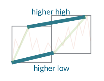
Trend Calculus is an algorithm invented by Andrew Morgan that is used to find trend changes in a time series (see here). It works by grouping the observations in the time series into windows and defining a trend upwards as “higher highs and higher lows” compared to the previous window. A downwards trend is similarly defined as “lower highs and lower lows”.
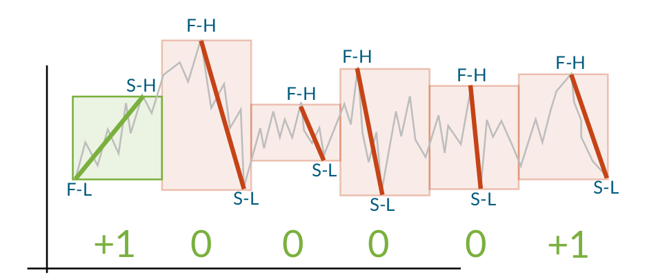
If there is a higher high and lower low (or lower high and higher low), no trend is detected. This is solved by introducing intermediate windows that split the non-trend into two trends, ensuring that every point can be labeled with either an up or down trend.
When the trends have been calculated for all windows, the points where the trends change sign are labeled as reversals. If the reversal is from up to down, the previous high is the reversal point and if the reversal is from down to up, the previous low is the reversal. This means that the reversals always are the appropriate extrema (maximum for up to down, minimum for down to up).
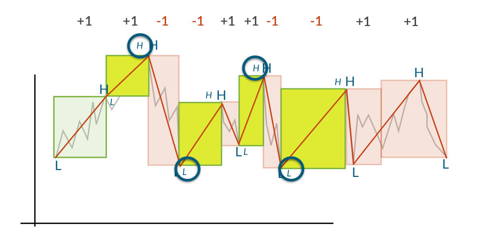
The output of the algorithm is a time series consisting of all the labelled reversal points. It is therefore possible to use this as the input for another run of the Trend Calculus algorithm, finding more long term trends. This can be seen when TrendCalculus is applied to the BCUSD datset, shown in column reversal1 of the table below.
val windowSize = 2
val numReversals = 1 // we look at 1 iteration of the algorithm.

val dfWithReversals = new TrendCalculus2(oilDS, windowSize, spark).nReversalsJoinedWithMaxRev(numReversals)
display(dfWithReversals)

val windowSpec = Window.orderBy("x")
val dfWithReversalsDiff = dfWithReversals
.withColumn("diff_close", $"y" - when((lag("y", 1).over(windowSpec)).isNull, 0).otherwise(lag("y", 1).over(windowSpec)))

// Store loaded data as temp view, to be accessible in Python
dfWithReversalsDiff.createOrReplaceTempView("temp")
In conjunction with TrendCalculus, a complete automatic trading pipeline can be constructed, consisting of (i) trend analysis with TrendCalculus (ii) time series prediction and (iii) control, i.e. buy or sell. Implementing and evaluating a pipeline such as the one outlined in the aforementioned steps is left as a suggestion for future work, and it is of particular interest to compare the performance of such a method to a learning-based one.
Below we show that sign(**diff_close**) is equivalent to sign of the output of a single iteration of TrendCalculus with window size 2, over our **scope**. A possible improvement of our algorithm would be to use TrendCalculus to compute long term trends from historical data and include it on our state definition. This way, if for example the agent observes a long term downward trend, then it can be encouraged to buy stock since it is bound to bounce up again.
# Taken from: https://lamastex.github.io/spark-trend-calculus-examples/notebooks/db/01trend-calculus-showcase.html

# Create Dataframe from temp data
fullDS = spark.table("temp")
fullTS = fullDS.select("x", "y", "reversal1", "diff_close").collect()

startDate = datetime.datetime(2019, 1, 1, 1, 0) # first window used as scope
endDate = datetime.datetime(2019, 1, 1, 23, 59)
TS = [row for row in fullTS if startDate <= row['x'] and row['x'] <= endDate]

allData = {'x': [row['x'] for row in TS], 'close': [row['y'] for row in TS], 'diff_close': [row['diff_close'] for row in TS], 'reversal1': [row['reversal1'] for row in TS]}

# Plot reversals
close = np.asarray(allData['close'])
diff_close = np.asarray(allData['diff_close'])
timesteps = np.linspace(1,len(diff_close),len(diff_close))
revs = np.asarray(allData['reversal1'])
pos_rev_ind = np.argwhere(revs ==  1)
neg_rev_ind = np.argwhere(revs ==  -1)
fig, ax = plt.subplots(2, 1, figsize=(16, 8))
ax[0].grid(True)
ax[0].plot(timesteps, close, label='close')
ax[0].plot(timesteps[pos_rev_ind], close[pos_rev_ind].flatten(), '*g', markersize=12, label='+ reversal')
ax[0].plot(timesteps[neg_rev_ind], close[neg_rev_ind].flatten(), '*r', markersize=12, label='- reversal')
ax[0].set_ylabel("close")
ax[0].set_xlabel("Timestep")
ax[0].set_xlim(1,len(close))
ax[0].legend()
ax[1].grid(True)
ax[1].plot(timesteps, diff_close, label='diff_close')
ax[1].plot(timesteps[pos_rev_ind], diff_close[pos_rev_ind].flatten(), '*g', markersize=12, label='+ reversal')
ax[1].plot(timesteps[neg_rev_ind], diff_close[neg_rev_ind].flatten(), '*r', markersize=12, label='- reversal')
ax[1].set_ylabel("diff_close")
ax[1].set_xlabel("Timestep")
ax[1].set_xlim(1,len(diff_close))
plt.tight_layout()
display(fig)
